Knot invariants of the SnapPy census knots

Abstract.

not too abstract

Table 1. Notational conventions used in this paper
[Sorted alphabetically by first column]

Common Objects
$D$	A knot diagram
$K$	A knot
$L$	A link
$M,N$	Manifolds
$\mathrm{\Sigma }$	A spanning surface of a knot
Numerical Invariants
$c(D)$, $c(K)$, $c(L)$	The crossing number of a diagram, knot, or link
$c{c}_3(K)$	The crosscap number for a knot $K$ in $S^3$
$ℳ𝒩(K),ℳ𝒩(L)$	The Morse–Novikov number of a knot, or link
$\mathrm{br}(K)$	The bridge number of a knot
$g_T(K)$	The Turaev genus
$s(K)$	The Rasmussen $s$-invariant
$\tau (K)$	The $\tau$-invariant
Polynomial Invariants
$J_K(n,t)$	The $n$-th colored Jones polynomial of a knot $K$
$J_K(t)$	The Jones polynomial of a knot $K$

NW: Question: Should we indicate above whether an invariant is used for a knot, link or diagram by writing $c(D),c(K),c(L)$ etc.? Yes

1. Introduction

While knot theory, the study of isotopy classes of embeddings $S^1\to S^3$, can be traced back to prehistoric times, its mathematical investigation began in the 19th century with the work of Gauss, Kelvin, and Tait [84, 226, 216]. The most natural and easiest way to present knots is via their diagrams. Apart from having an actual $3$-dimensional model of a knot in space, a knot diagram is the most natural way to study and analyze knots.

Therefore, it might not be surprising that knots have been tabulated and ordered for centuries according to the complexity of their diagrams in terms of their crossing numbers [215, 141, 142, 143, 54, 43, 185, 189, 220, 105, 106, 37, 225]. The current state of the art are Burton’s and Thistlethwaite’s papers [37, 225] that classify all knots with at most 20 crossings. Furthermore, in the last decades, the combined work of the mathematical community has yielded to the computation of most invariants for the low-crossing knots. These computations have been collected at single places (most notably KnotInfo [144, 44] and Knot Atlas [21], but we also mention [206]) to form databases that turned out to be extremely useful for research in the last years. For example, KnotInfo was cited (due to Google Scholar at the time of writing) more than 500 times since its creation in 2011.

On the other hand, the approach of studying knots via their diagrams is somehow known to be the wrong perspective on knot theory for several reasons. Many typical properties and behaviors cannot (or only very rarely) be seen for low-crossing knots so we might get wrong impressions of general behavior by considering only low-crossing knots. In general, it remains also mysterious which properties of a diagram actually represent properties of the knot and vice versa.

The more fruitful approach pioneered in the last decades by ingenious work of many mathematicians, including Thurston [227], Gordon–Luecke [88], Haken [97], Weeks [234], Lackenby [133, 134], and Coward–Lackenby [55] to only mention a few, is to consider instead of a diagram the complement of a knot. Modern knot theory often studies the complement of a knot with techniques from $3$-manifold topology to answer questions about knots (and in particular also about their diagrams).

In that light, it might be natural to also enumerate knots according to the complexity of their complement. Here a natural complexity is the minimal number of tetrahedra needed to ideally triangulate the complement. Dunfield [72], cf. [40], has tabulated all hyperbolic knot complements that can be built by gluing together at most $9$ ideal tetrahedra. These $1267$ knots are called census knots. This was done by classifying all exceptional slopes of the 1-cusped hyperbolic manifolds in the SnapPy census [102, 41, 36] and reading off which of those admit $S^3$-fillings. However, due to its construction, the census knots do not come with any diagrams and thus it is not clear how to compute knot invariants or determine other properties of the census knots that require diagrams.

In recent work [16] we have written Python code that created knot diagrams of all census knots. For an alternative proof see [190]. In fact, we can see that many of these knots have no known diagrams with crossing numbers less than $200$. This generalizes our previous work on the asymmetric census knots [9] and the older work in [39, 46, 45]. We expect the census knots to capture different phenomena and behavior than the low-crossing knots. In fact, we could already use the diagrams of the census knots to verify the existence of a hyperbolic L-space knot that is not braid positive [16] and answer some other open questions.

The goal of this paper is to announce computations of knot invariants of the census knots. We hope that these data will be useful for other research projects. All the data can be accessed online at the webpage to add. The computations were mainly done by using the standard programs for low-dimensional topology: SnapPy [61], Regina [34], their combination in SageMath [95, 194] and Mathematica [109]. In addition, all the code is available at the GitHub repository to add.

In the rest of this introduction, we will summarize our results and discuss questions and observations we made while studying the knot invariants of the census knots. In the main body of this paper, we will quickly discuss the invariants, and the available methods of their computations, and provide references. We hope that this document will be useful for researchers in knot theory looking for methods to explicitly compute knot invariants.

The rest of the introduction needs to be added later.

1.1. Computed invariants

1.2. New results

1.3. Verified conjectures

1.4. Curiosities, question and observations

Acknowledgements

We have received help from numerous other mathematicians on this project. We would like to express our sincere thanks to all of them.

Special thanks to the creators of KnotInfo, Charles Livingston and Allison H. Moore, for their assistance in creating the website and especially for sharing their code on which our website is based. Need to include their founding…

Furthermore, we thank Fabio Gironella, add the others for their help in starting this project, Tatiana Levinson for writing the code that was used for computing the signature functions, Juan González-Meneses and Marithania Silvero for their help in obstructing the final knots from being braid-positive and useful discussions, Mark C. Hughes and Justin Meiners for running their code to find quasi-positive braid words for some knots, Lukas Lewark for useful comments, and Jonathan Spreer for sharing his code for computing the crosscap numbers and interesting related discussion.

Miguel Marco for help with homflypt

TO DO: Add founding: BMS, ICERM,…

Add Datenstation HU Berlin

Peter Feller has found a SQP braid word of minimal braid index of $m(09\mathrm{\_}39519)$.

Adrian Dawid

2. Nomenclature [Marc - done]

should explain prime decomposition theorem

As mentioned in the introduction, knots are collected in various tables, sorted, and named in different ways. Here we mention the most common ways to do so. Since every knot uniquely decomposes into prime summands [197] these lists only contain prime knots. On top of that there exist knots that are not isotopic to their mirror images. (The simplest such knot is the trefoil.) Thus these tables only list one chirality of the knots.

Since the decision problem for $3$-manifolds is solved [132] and since knots are determined by their exteriors [88] we can algorithmically determine if a given knot appears in one of the tables. In practice, we use SnapPy to search for an isometry and if we cannot find such an isometry we use the verified volume (see Section 7.1) to distinguish knots. The results in Sections 2.1–2.4 are verified to be complete, however, the results in Section 2.5 might be incomplete since the verified volumes of the knots in Burton’s list was not computed for all (i.e. there might be census knot with crossing number $18$ or $19$ that are in Burton’s list but do not appear in our list).

2.1. SnapPy tetrahedral census name

Any cusped finite volume hyperbolic $3$-manifold can be triangulated using ideal tetrahedra. The SnapPy census [102, 41, 36] consists of all cusped finite volume hyperbolic $3$-manifolds that can be triangulated by at most $9$ ideal tetrahedra. For example, the figure eight knot can be triangulated by gluing together two ideal tetrahedra [227]. In the SnapPy census, the figure eight knot is named $m004$. Here the first letter gives the number of tetrahedra. Here $m$ means that the number of tetrahedra is at most $5$. If the first letter is $s$, $v$, $t$, or $o9$, this means that the manifold can be triangulated by $6$, $7$, $8$, or $9$ tetrahedra, respectively. The second number displays the lexicographical order among the manifold with the same letter, where we first order by volume and then by the lengths of the shortest geodesics.

2.2. Census knot name

Dunfield [72], cf. [40], has tabulated all knot complements in the SnapPy census. These $1267$ knots are called census knots. In the census knot notation the figure eight knot is named $K2\mathrm{\_}1$, where the $K2$ indicates that its complement can be triangulated by $2$ ideal tetrahedra (and not with fewer) and the second number is given by the order induced from the order of the tetrahedral census (based on the volume and the lengths of the shortest geodesics).

2.3. Rolfsen name

In [189] Rolfsen has published a list of all prime knots with diagrams of at most $10$ crossings. In this notation, the figure eight knot is named by $4\mathrm{\_}1$, where the first number gives the crossing number of the knot at hand. The second number is an index among knots with the same crossing number, where always the first knots are torus knots followed by twist knots. Also, the alternating knots are listed before the non-alternating knots. However, apart from this, the numbering seems to be arbitrary.

Rolfsen’s list is based on the earlier lists by Alexander–Briggs [7] and Conway [54] where a few errors have been corrected. However, neither the completeness nor the correctness of these lists were rigorously verified (as also remarked by Rolfsen himself in the footnote on Page 388 in [189]). And in fact, it turned out later that Rolfsen’s original list contained a double, the so-called Perko pair, as noticed by Perko [185]. The knots $10\mathrm{\_}161$ and $10\mathrm{\_}162$ (in Rolfsen’s original numbering) are in fact isotopic. There are different ways to resolve that mistake. Some people just deleted $10\mathrm{\_}162$ and kept the indices of the other knots the same, in other sources the numbering was changed (and in some sources, the mistake was just kept). Unfortunately, there is not a commonly agreed way to resolve that issue. This has yielded to further mistakes [236, 75]. For other smaller mistakes and inconsistencies in Rolfsen’s original list, we refer to [206].

The first rigorous proof that this list is complete and correct was given when classifying all knots with at most $16$ crossings by computer methods in [105] using the DT notation, see below. Here we follow the obvious solution (which is unfortunately only used by a minority of researchers in the field) and just do not use Rolfsen notation but instead use the DT notation when we want to refer to low-crossing knots. This is not just completely avoiding inconsistencies that appear when using the Rolfsen notation, or using a mix of notations when discussing knots with higher crossing numbers, but also gives credit to the researchers that first developed and implemented rigorous methods to tabulate knots.

2.4. DT name

The DT name of a knot is based on the Dowker–Thistlethwaite notation [70] of knot diagrams (see Section 2.4). The DT notation together with the solutions of the various Tait conjectures [215, 121, 163, 162, 221, 223, 93] can be used to effectively and rigorously enumerate all prime knot diagrams up to a certain crossing number. In the second step, one searches for isotopies of the knots represented by these diagrams to group them into sets of diagrams representing isotopic knots. In the last step, one computes knot invariants to show the correctness of the list from the previous step. This approach was done independently with slightly different methods (especially in the choice of invariants to distinguish knots) by different sets of authors and programs [105, 37, 225]. It turns out that all these classifications agree and thus are most likely correct. Currently, all prime knots with crossing number at most $20$ are classified.

The DT name of the figure eight knot is $K4a1$. Here the $K4$ tells us that it is a knot with crossing number $4$. The second letter is either $a$ or $n$ indicating if the knot is alternating or non-alternating. The last number is an index based on the lexicographical ordering of the minimal DT notation of the knot [70].

2.5. Burton name

The notation of Burton [37] displays more information about the knots. The figure eight knot in Burton’s notation is $4ah\mathrm{\_}1$. In general, the name is of the form $c[a/n][t/s/h]\mathrm{\_}i$, where the first number $c$ is the crossing number, the second entry indicates whether the knot is alternating or non-alternating, the third entry tells us if the knot is a torus, satellite or hyperbolic knot and the last entry is an integer that sorts the knots within each of these classes by the structure in the non-hyperbolic case and roughly by volume in the hyperbolic case.

3. Presentations

In this section, we should discuss which programs can compute which presentations and take what as input.

3.1. Braid word [Marc - done]

Braids were introduced in the work of Artin [11, 10]. An $n$-braid $b$ consists the isotopy class of $n$ disjoint properly embedded intervals $c_i$, for $1\le i\le n$, in a cylinder $[0,1]\times D^2$ with endpoints in $(0,0,i/(n+1))$ and $(1,0,\sigma (i)/(n+1))$ and such that the first coordinate is strictly increasing. Here $\sigma$ is some permutation of $[1,\mathrm{\dots },n]$ that depends on the braid $b$. An example is shown in Figure 1.

One can multiply two $n$-braids $b_1$ and $b_2$ by gluing the right part of the braid $b_1$ to the left part of the braid $b_2$. This makes the set $B_n$ consisting of all $n$-braids into a group with neutral element the $n$-braid consisting of $n$ straight lines (of constant $z$-coordinates). Algebraically, the braid group is generated by, the so-called Artin generators. The $i$-th Artin generator ${\sigma }_i$, for $i\in \{1,\mathrm{\dots },n-1\}$, is the $n$-braid that consist of just straight lines except the lines $i$ and $i+1$ (counted from top to bottom) which make a half right-handed twist. Each braid can be presented by a word in the ${\sigma }_i$ and their inverses.

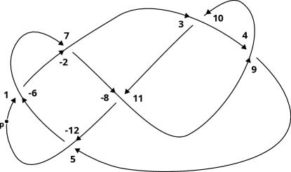
We use the notation as for example used in SnapPy [61] which presents a braid word as a list of integers, where the natural numbers present the Artin generators and the negative numbers their inverses. We refer to Figure 1 for an example.

Figure 1. Left: A $4$-braid with braid word $[1,-2,3,-2,1,-2,1,3]$. Right: A diagram of its closure.

define index of a braid

Braids are closely related to knots and links. From a given braid one can form its closure by connecting the endpoints of the braid as shown in Figure 1 to create a link. Alexander [8] has shown that any link arises as the closure of a braid. Although the braid presentation is not unique. Markow has described exactly which braids have isotopic closures [150].

Further information on braids can for example be found in [24, 186].

We list for any census knot a braid word. The braid words were first constructed in [16]. We have always tried to display a braid word of minimal index and if possible one that is (strongly / quasi) positive or negative, if such a word exists. Note that there exist braid positive knots such that no positive braid word has minimal braid index [158]. However, among the census knots we could not find such an example. Although the computations of all braid indices is not finished.

Mention other ways to present braids. For example alphabetical.

3.2. PD code [Leo]

A Planar Diagram (PD) code (resp. notation) of a link diagram is a list of 4-tuples of integers from which the link diagram can be recovered. origin of this notation Given a link diagram $D$, a PD code can be obtained as follows:

Pick a starting point on the link in the diagram. Now go along the orientation of the link component on which the point was chosen and label the edges (starting with 0) each time the link component goes over or under a crossing. Now further label the edges by choosing a point on a different component and repeating this process. Now for each crossing, a 4-tuple is obtained by listing the label on each edge starting with the incoming lower edge and going counterclockwise, see Figure X for an example. Therefore each integer appearing in the PD code corresponds to an edge, and each 4-tuple corresponds to a crossing.

Conversely, such a PD-code determines a link diagram.

Figure 2. Obtaining a PD-code of a diagram of the negative trefoil: $[(1,5,2,6),(3,1,4,6),(5,3,6,2)]$

Many mathematical software programs, like SnapPy, Sage, add more? which work with links can create a link diagram given a PD code and can also return a PD code of a given link diagram.

We also want to mention Knotfolio, a browser-based program for drawing and manipulating knots and links, which can generate a PD code given a drawing or a picture of a link diagram. add citation

left to do: add citations, make example figure nice, add the origin of this notation

3.3. DT code [Nicolas, Open for Review]

The Dowker–Thistlethwaite (DT) code (resp. notation) for a knot diagram was introduced by Dowker and Thistlethwaite in [69] where they proved that for prime knots, the knot can be recovered from the DT code up to reflection. To see that chirality detection fails simply consider the trefoil, see Figure 4 where in both cases the DT code will be $[4,5,6]$ when starting the traversal in the same way as indicated in the figure. Why does it not work for connected sums? NW: The wikipedia article points out that if we have have connected sums then there is the chirality issue for each component. that should maybe be briefly discussed

To obtain it, fix an orientation of the knot diagram, and, in order of traversal, label each crossing by $1,\mathrm{\dots }2n$, where $n=c(K)$ is the number of crossings. Note that each crossing receives both an even and an odd label, which is clear when considering the partial traversal starting and ending at a fixed crossing.

Now, add a negative sign to each even label at an over-crossing. Ordered by the odd part, one obtains the sequence of labels $(1,e_1),\mathrm{\dots },(2n-1,e_{2n-1})$. The DT code of the diagram is then obtained by collecting the even labels in the order of the odd parts. The diagram in Figure 3 illustrates the procedure.

Figure 3. A knot diagram with DT code $[\text{-}6,10,\text{-}12,\text{-}2,4,\text{-}8]$

See also Section 2.4 on the DT name.

3.4. (Extended) Gauss code [Nicolas, Done - Open for Review]

The Gauss code of a diagram is obtained by labelling the vertices, each only once, in some order of traversal and then noting down their occurrence always with a sign denoting over- resp. under-crossing. As it doesn’t additionally capture the orientation of crossings it also cannot distinguish chiral knots. See Figure 4 for the example of the trefoil knot.

Figure 4. Both the left- and right-handed trefoil knot can be described by the Gauss code $[1,\text{-}2,3,\text{-}1,2,\text{-}3]$. For the extended Gauss code we have $[1,\text{-}2,3,\text{-}1,\text{-}2,\text{-}3]$ on the left and $[1,\text{-}2,3,1,2,3]$ on the right.

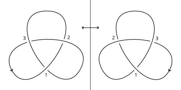
To be able to reconstruct the knot diagram exactly, one may use the extended Gauss code. After labelling the crossings as before, one then records the label on each first visit with the sign $\pm 1$ for an over vs under crossing. On the second visit, the sign $\pm 1$ denotes a left- vs. right-handed crossing. We refer again to Figure 4 for illustration.

4. 3-dimensional properties

4.1. Alternating [Jan - Updated March 24]

An alternating diagram of a knot, is a diagram where over and under crossings alternate as we move along the projection of the knot. A knot is called alternating if there exists an alternating diagram for this knot. It has long been an open question, whether there exists a non-diagramatic description of alternating knots. Recently, two independent works [92, 107] provided a topological characterisation of alternating knot exteriors positively answering the above question. Both works also provide practical algorithms to determine whether a knot is alternating based on a triangulation of the knot exterior. Maybe we should also mention the tait conjecture and that this yields an algorithm just using the decision problem. We did not make use of this algorithm as the implementation is not straightforward.

We determined the alternating status of census knots in a 2-step approach, first we searched for alternating diagrams using SnapPy [61]. We randomly modified known diagrams of census knots, simplified the diagrams and then checked whether they are alternating. It is known that reduced? alternating diagrams have minimal crossing numbers among all diagrams of a knot [164, 222, 122], which is why we simplify the diagrams before checking the alternating status. For the remaining knots, we then tried to find obstructions to being alternating. The most useful in our case was the connection between the Alexander polynomial and knot Floer homology for alternating knots detailed below.

Theorem 4.1 (Theorem 1.3 in [177])

Given a knot $K\mathrm{\subset }{S}^{\mathrm{3}}$, its signature $\sigma$, and its symmetrized Alexander polynomial

$${\mathrm{\Delta }}_K(t)=a_0+\sum _{s>0}{a}_s(T^s+T^{-s}),$$

its knot Floer homology is supported only in dimensions $s\mathrm{+}\sigma \mathrm{/}\mathrm{2}$, i.e. it is homologically $\sigma$-thin, and given by

For knots with known knot Floer homology, we then checked whether the Alexander polynomial and knot homology satisfy the above equivalence. Knots whose invariants do not satisfy this equivalence cannot be alternating. An analogous result also holds for the Khovanov homology and the Jones polynomial

Theorem 4.2 ([148])

Given a knot $K\mathrm{\subset }{S}^{\mathrm{3}}$, its signature $\sigma$, and its Jones polynomial

$$J_K(t)=\sum _k{a}_k{t}^k,$$

its reduced Khovanov homology is supported only in dimensions $s\mathrm{+}\sigma \mathrm{/}\mathrm{2}$, i.e. it is homologically $\sigma$-thin, and given by

Finally we also made use of the following theorem

Theorem 4.3 (Theorem 1.5 in [180])

If $K\mathrm{\subset }{S}^{\mathrm{3}}$ is an alternating L-space knot, the it is a $\mathrm{(}\mathrm{2}\mathrm{,}\mathrm{2}\mathit{}n\mathrm{+}\mathrm{1}\mathrm{)}$ torus knot for some integer $n$.

All census knots are hyperbolic and thus cannot be torus knots. This implies that all L-space census knots cannot be alternating. Since the L-space status of census knots was already computed in [9], we could exclude further knots from being alternating. Other properties of alternating knots which can used as obstructions are the following

• The Seifert genus of an alternating link is the degree of the symmetrized Alexander polynomial and a Seifert surface obtained from applying Seiferts algorithm to an alternating diagram realizes the Seifert genus [161, 60].

• The writhe of an alternating knot is a knot invariant, and amphichiral alternating knots have zero writhe [223].

4.2. Quasi-alternating [Marc - done]

Quasi-alternating links are defined recursively as follows. The set of quasi-alternating links $QA$ is the smallest set of links such that

1. the unknot is in $QA$, and

2. if a link $L$ has a crossing $c$ in a diagram $D$ such that both smoothings $D_0$ and $D_1$ at $c$ represent links $L_0$ and $L_1$ in $QA$ with $det(L_0)+det(L_1)=det(L)$, then $L$ is also in $QA$.

This notion generalizes alternating links since any non-split alternating link is quasi-alternating [174]. Its importance stems from the result that the double branched cover branched along a quasi-alternating link is a Heegaard Floer L-space [174]. On the other hand, there exist quasi-alternating knots that are not alternating [144], thin knots that are not quasi-alternating [90], cf. [89], and thick (i.e. non-thin) knots whose double branched covers are L-spaces, see for example [110]. Other infinite families of non-split thick knots whose double branched covers are L-spaces are given in [14].

For the census knots, we could completely determine which are quasi-alternating and which are not. To show that a knot is quasi-alternating, we have first used the available information on low-crossing knots [144, 114] and then have searched recursively via the definition for a quasi-alternating description. The latter works well, if the knot at hand has a diagram with relatively few crossing but did not work well if the knots had many crossings. Other ways to construct quasi-alternating knots are given in [48, 50].

As obstructions, we have used the following results:

Theorem 4.4 (Manolescu–Ozváth [147], Ozváth–Rasmussen–Szabó [176])

If $K$ is quasi-alternating then it is Khovanov homology and knot Floer homology thin. (And also thin in even Khovanov homology.)

Here a link is called thin if the corresponding (reduced) homology theory is supported in only two (one) diagonals. From the spectral sequence relating Khovanov homology and knot Floer homology [71] it follows that a knot Floer thin link is also Khovanov thin.

Theorem 4.5 (Baldwin [20])

If $K$ has braid index $\mathrm{2}$ or $\mathrm{3}$ then $K$ is quasi-alternating if and only if it is Khovanov homology thin.

Theorem 4.6 (Teragaito [217], Chbili–Qazaqzeh [188])

If $K$ is quasi-alternating then $\mathrm{deg}\mathit{}\mathrm{(}{Q}_K\mathrm{)}\mathrm{\le }\det \mathrm{(}K\mathrm{)}\mathrm{-}\mathrm{1}$ ($\mathrm{\le }\det \mathrm{(}K\mathrm{)}\mathrm{-}\mathrm{2}$ if $K$ is not a torus knot), where $Q_K$ is the $Q$-polynomial.

In our normalization the $Q$-polynomial is given by $Q_K(z)=F_K(1,z)$ for $F$ the Kauffman polynomial, see Section 9.5.

Theorem 4.7 (Teragaito [218])

If $K$ is quasi-alternating then ${\mathrm{deg}}_z\mathit{}\mathrm{(}{F}_K\mathrm{)}\mathrm{\le }\det \mathrm{(}K\mathrm{)}\mathrm{-}\mathrm{1}$ ($\mathrm{\le }\det \mathrm{(}K\mathrm{)}\mathrm{-}\mathrm{2}$ if $K$ is not a torus knot), where $F_K$ is the Kauffman polynomial.

Theorem 4.8 (Teragaito [219])

If $K$ is quasi-alternating then $\mathrm{deg}\mathit{}\mathrm{(}{Q}_K\mathrm{)}\mathrm{\le }{\mathrm{deg}}_z\mathit{}\mathrm{(}{F}_K\mathrm{)}\mathrm{\le }\det \mathrm{(}K\mathrm{)}\mathrm{-}\mathrm{3}$.

Theorem 4.9 (Lidman–Sivek [139])

If $K$ is quasi-alternating and hyperbolic with $\det \mathrm{(}K\mathrm{)}\mathrm{\le }\mathrm{7}$ then $K$ is a $\mathrm{2}$-bridge knot (and in particular alternating).

Theorem 4.10 (Khovanov [126])

If $K$ is adequate and not alternating then $K$ is Khovanov homology thick and thus not quasi-alternating.

Theorem 4.11 (Issa [110])

Quasi-alternating Montesinos knots are classified.

Theorem 4.12 (Boileau–Boyer–Gordon [26])

If $K$ is braid positive then $K$ is Khovanov homology thick and thus cannot be quasi-alternating.

Other obstructions from the Jones polynomial and related invariants are given in [51]. Further results can be found in [219]

4.3. Almost alternating [Jan]

A knot K is called almost alternating, if it is not alternating and has a diagram D which can be transformed into an alternating diagram by a crossing change. Note that being almost-alternating is equivalent to having having Turaev genus 1 [63]. Also do we want almost alternating or almost-alternating? I chose almost alternating to be consistent with knot info. By the definition above we can exclude all alternating knots from being almost-alternating. Another obstruction is given by the Jones polynomial. are there other obstructions? i havent found any others, but will have another look

Theorem 4.13 (Thm 1.3 from [66])

Given an almost alternating link L and its Jones polynomial

$$J_L(t)=\sum _{i=m}^n{a}_i{t}^i$$

with $a_n\mathrm{\ne }\mathrm{0}\mathrm{\ne }{a}_m$, then either $\mathrm{|}{a}_m\mathrm{|}\mathrm{=}\mathrm{1}$, $\mathrm{|}{a}_n\mathrm{|}\mathrm{=}\mathrm{1}$ or both.

We can look for almost alternating knots by starting with a diagram D, changing a crossing and checking if the resulting diagram is alternating. This can be repeated for all crossings of the diagram D. For a given knot K, one can also use different diagrams D for the search.

4.4. Adequacy [Nicolas]

The class of adequate knots form an extension of the alternating knots. They are similarly defined via the existence of an adequate diagram which realizes the knot. In particular, adequate diagrams realize the crossing number of the knot, see for example [224]. Conversely, a minimal diagram of an adequate knot is adequate. They were introduced by Lickorish and Thistlethwaite in [138]. Are there examples of adequate knots that are not alternating?

4.4.1. Definition

Given a crossing in a diagram, we may consider its positive (also A or leftwards) respective the negative (also B or rightwards) resolution from the perspective of the over-crossing strand as depicted in Figure 5.

Figure 5. The two orientation-independent resolutions of a crossing

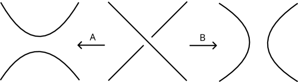
This definition is independent of a choice of orientation. After applying any type of resolution to all of the crossings one obtains a collection of planar, disjoint $S^1$’s. The behaviour of the number of these circles under different resolutions leads to the definition of adequacy. Observe also that the number of circles must necessarily change when the resolution of a crossing is changed.

Definition 4.14

Given a knot diagram, we call it positively adequate if its positive resolution is maximal. In other words, changing the resolution of any crossing decreases the number circles. Similarly, it is called negatively adequate if its negative resolution is maximal.

A knot diagram is called adequate if it is both positively and negatively adequate.

A knot is called adequate if it admits an adequate diagram.

Note that the above definition translates mot à mot to the setting of links.

4.4.2. Characterization of Adequacy and Obstructions

In [2], Abe relates Turaev genus of an adequate knot to the width of its Khovanov homology, culminating in the following theorem:

Theorem 4.15

[2, Thm. 3.2] Let $K$ be a knot with an adequate diagram $D$, then

$$g_T(K)=g_T(D)=1/2(c(D)-|s_{+}D|-|s_{-}D|)+1={\omega }_{\text{𝐾ℎ}}(K)-2=c(K)-\text{𝑠𝑝𝑎𝑛}{V}_K(t).$$

In the above theorem, $g_T$ denotes the Turaev genus, $c(-)$ the crossing number, $|s_{+}D|$ and $|s_{-}D|$ the number of circles in positive respective negative resolution, and $V_K(t)$ the Jones polynomial.

Later, in [119] Kalfagianni presents a complete characterization adequate knots in terms of the colored Jones polynomial $J_K(n,t)$.

Theorem 4.16

[2, Thm. 1.1] Let $K$ be a knot an $J_K\mathit{}\mathrm{(}n\mathrm{,}t\mathrm{)}$ its colored Jones polynomial of degree $n$. Then, by [83] we have

$${\text{𝑠𝑝𝑎𝑛}}_t{J}_K(n,t)=s_1(n)n^2+s_2(n)n+s_3(n)$$

where the $s_i\mathit{}\mathrm{(}n\mathrm{)}$ are periodic for $n$ larger than some $n_K$.

Then $K$ is adequate if and only for some $n\mathrm{>}{n}_K$, we have

$$s_1(n)=c(K)/2\mathit{\text{ and }}{s}_2(n)=1-g_T(K)-c(K)/2.$$

Furthermore, every diagram of $K$ that realizes $c\mathit{}\mathrm{(}K\mathrm{)}$ is adequate and it also realizes $g_T\mathit{}\mathrm{(}K\mathrm{)}$.

4.4.3. Adequacy Results

There are $81$ census knots know to be alternating and hence also adequate. NW: Is alternatingness known for all? yes, that should be discussed in that section Further $588$ census knots were obstructed from being adequate via the result by Abe on the Turaev genus and the Khovanov width.

Finally, we did not make use of the Jones slopes characterization by Kalfagianni as the computation of the colored Jones polynomials still appears infeasible for the census knots.

4.5. Homogenicity [Nicolas, Done - Open for Review]

Homogenicity was originally defined by Cromwell in [58] for links, even though here we phrase everything in terms of knots: We first define homogenicity of knot diagrams as homogenicity of their Seifert graph which then gives the criterion for a knot to be homogeneous:

Definition 4.17

Homogenicity is first defined as a property of a graph with signed edges. Decompose $G$ first into its blocks by cutting along all cut vertices of $G$. If $v$ is a cut vertex and $G_1,\mathrm{\dots },G_k$ are the connected components of $G-v$, then the result of cutting at $v$ is the collection of subgraphs $G_1\cup v,\mathrm{\dots },G_k\cup v$ where the edges in ${\{v\}\times V|}_{G_i}$ are adjoint as well. The graph $G$ is then call homogeneous if all its blocks only contain edges of the same sign.

For a knot diagram, consider the Seifert surface obtained via the Seifert algorithm [201]. The way its obtained is encoded in the Seifert graph $G=(V,E)$. Consider as vertices the Seifert disks enclosed by the crossings. The signed edges correspond to the crossings along which the disks are glued, the sign representing the sign of the crossing.

NW: In case the Seifert graph is defined somewhere already before, then add a reference to that section.

A knot diagram is then called homogeneous if its Seifert graph is homogeneous. A knot in turn is called homogeneous if it admits a homogeneous diagram.

4.5.1. Conditions and Obstructions for Homogenicity

For the Census knots we have been able to determine the homogenicity status for $990$ out $1267$ knots. The obstruction and characterizations we used in this process are mainly from Cromwell’s original paper and we will shortly mention them below.

Every positive knot is homogeneous for the simple reason that its Seifert graph will only contain positive edges. It was also shown by Baader in [12] that homogenicity is the link between positivity and strong quasipositivity. Later Abe generalized in [4] to the following characterization of positivity, relating it furthermore to the $\tau$-invariant, Rasmussen $s$-invariant, and $3$-genus $g_3$ and smooth $4$-genus $g_4$.

Theorem 4.18 ([4, Thm 1.3.])

Let $K$ be a knot. Then (1)-(4) are equivalent.

1. $K$ is positive.

2. $K$ is homogeneous and strongly quasipositive.

3. $K$ is homogeneous, quasipositive and $g_4(K)=g(K)$.

4. $K$ is homogeneous and $\tau (K)=s(K)/2=g_4(K)=g(K)$.

NW: Should we place this here or link to positivity? both

Cromwell does also observe that alternative knots, which were defined by Kauffman in [120] and generalize alternating knots, are homogeneous too.

The main part of Cromwell’s paper then amounts to studying properties of homogeneous links. In particular, we mention the following two that were useful for us, where $P(L)(v,z)$ denotes the HOMFLY polynomial of a link $L$ and $\nabla (L):=P(1,z)$ is its Conway polynomial.

Theorem 4.19 ([58, Thm. 4])

Let $L$ be a homogeneous link and let $\chi \mathit{}\mathrm{(}L\mathrm{)}$ denote the maximal Euler characteristic over all orientable surfaces spanning $L$. Then

1. ${\text{𝑚𝑎𝑥𝑑𝑒𝑔}}_{z}P(L)=1-\chi (L)$

2. ${\text{𝑚𝑖𝑛𝑑𝑒𝑔}}_{v}P(L)\le 1-\chi (L)$ with equality if and only if $L$ is positive.

Theorem 4.20 ([58, Cor 5.1, Cor 5.2])

If $L$ is a homogeneous link and the leading coefficient of $\mathrm{\nabla }\mathrm{(}L\mathrm{)}$ is $\mathrm{\pm }\mathrm{1}$ then $L$ has order at most $\mathrm{2}\mathrm{\cdot }\text{𝑚𝑎𝑥𝑑𝑒𝑔}\mathit{}\mathrm{\nabla }\mathrm{(}L\mathrm{)}$.

Furthermore, for a homogeneous link the leading coefficient of $\mathrm{\nabla }\mathrm{(}L\mathrm{)}$ is $\mathrm{\pm }\mathrm{1}$ if and only if $L$ is fibered.

Eventually, Cromwell presents the list of non-alternating homogeneous prime knots up to order $10$ with the exception of five knots. For them their status was determined by Stoimenov in his paper on knots of genus two [205].

4.5.2. Homogenicity results

The above results allowed us to determine and obstruct homogenicity for $990$ knots as follows:

1. $787$ (NW: Is this the currently correct number?) census knots are known to be positive.

2. $46$ census knots are alternating, hence alternative.

3. $9$ non-alternating homogeneous Census knots are found in the list of Cromwell.

4. For $80$ census knots, homogenicity was obstructed by the knowledge of the HOMFLY polynomial and the Euler characteristic respectively $3$-genus.

5. A further $67$ knots were obstructed by the corollary on the Conway polynomial.

6. The positivity characterization of Abe obstructed $1$ further Census knot.

Note most of the obstructions above used either directly or indirectly the HOMFLY polynomial which he have not yet determined for all knots (NW: correct?) or relied on bounds of the $4$-genus or crossing number. We assume that determining these missing invariants or having better bounds will allow for obstructing homogenicity for further knots.

4.6. 2-Bridge and Montesinos knots [Marc - done]

$2$-bridge links were defined and classified by Schubert [199], who attributed it to Seifert. They are known to be exactly the links in $S^3$ whose double branched covers are lens spaces. Any $2$-bridge link is alternating by [54].

A generalization of $2$-bridge links are Montesinos links [154], the links in $S^3$ whose double branched covers are Seifert fibered spaces [238]. For detailed information and more literature on $2$-bridge and Montesinos links we refer to [33, Chapter 12]. Every pretzel or $2$-bridge link is a Montesinos link.

For determining if a given knot $K$ is a $2$-bridge or Montesinos knot and determining their $2$-bridge and Montesinos notations we proceed as follows.

• We use SnapPy to build the double branched cover $\mathrm{DBC}(K)$ branched along $K$.

• We use SnapPy inside Sage to try to verify that $\mathrm{DBC}(K)$ is hyperbolic. If this is the case, $K$ is not a Montesinos or $2$-bridge knot.

• If SnapPy does not succeed in verifying the hyperbolicity of $\mathrm{DBC}(K)$, we apply Dunfield’s recognition code [72] (using the combined power of regina and SnapPy) on $\mathrm{DBC}(K)$.

• If this recognizes $v$ as a Seifert fibered space we know that $K$ is a Montesinos knot and from the Seifert invariants of $\mathrm{DBC}(K)$ we can read off the Montesinos notation of $K$. Here a Seifert fibered space

  $$SFS[S2:(2,1)(3,1)(7,-6)]$$

  in regina’s notation corresponds to the Montesinos invariants

  $$(1,2),(1,3),(-6,7).$$

• If $\mathrm{DBC}(K)$ is the lens space $L(p,q)$, $K$ is the $2$-bridge knot $K(p/q)$.

• If $\mathrm{DBC}(K)$ is a JSJ manifold, $K$ is not a Montesinos knot. (But if $\mathrm{DBC}(K)$ is a graph manifold, $K$ is an arborescent knot.)

For the census knots, this was enough to determine the type of all double branched coverings. In total, we have:

• $77$ knots have lens space double branched coverings and thus they are $2$-bridge,

• $114$ have other Seifert fibered spaces as double branched coverings and they are Montesinos knots,

• $9$ have graph manifolds double branched coverings and the knots are arborescent knots,

• $6$ have as double branched coverings a JSJ manifold, and

• all $1061$ remaining knots have hyperbolic double branched coverings.

4.7. Large or Small [Nicolas, Done - Open for Review]

Definition 4.21 (Large and Small Knots)

We call a knot $K$ in $S^3$ large if its exterior $M$ (the complement of an open tubular nhd of $K$) contains a closed essential surface.

For completeness we define essentiality of a properly embedded surfaces in a compact orientable irreducible $3$-manifold with boundary following [202]. Immediately afterwards we specialize to knot exteriors in $S^3$.

Definition 4.22 (Essential Surface)

In the context mentioned above, a properly embedded non-empty connected surface $\mathrm{\Sigma }\hookrightarrow M$ is called essential if it satisfies:

1. $\mathrm{\Sigma }$ is bicollared.

2. The induced morphism $\pi (\mathrm{\Sigma })\to \pi (X)$ is injective (i.e. $\mathrm{\Sigma }$ is an injective surface).

3. $\mathrm{\Sigma }$ is not boundary-parallel.

4. $\mathrm{\Sigma }$ is not a sphere.

Note that one then also may define a compact orientable irreducible $3$-mfld to be Haken if it contains an essential surface. Then every knot exterior is Haken by means of a minimal genus Seifert surface. The condition to be large, however, is stronger. Not every knot exterior contains a closed essential surface.

Also note that if we restrict our attention to knot exteriors, the definition of a closed essential surface simplifies as follows, where injectivity is also equivalent to incompressibility:

Definition 4.23 (Closed Essential Surfaces in Knot Exteriors in $S^3$)

A closed essential surface $\mathrm{\Sigma }$ in the knot exterior $M$ of $K\hookrightarrow S^3$ is an orientable, embedded, injective and not boundary-parallel closed surface of positive genus.

4.7.1. Algorithms for computing closed essential surfaces

A first algorithm for testing for the existence of closed essential surfaces in compact irreducible closed $3$-manifold $M$ was provided Jaco and Oertel in [115] in 1984. This algorithm works with a handle body structure of $M$, constructs candidate surfaces using normal surface theory and then test for injectivity by checking incompressibility of the double of the respective surface.

In 2012 Burton, Coward, and Tillmann in [35] then discuss an improved algorithm for computing closed essential surfaces in knot exteriors respectively knot complements, which allows for extension to other kinds of 3-manifolds as they point out and then later discuss in [38]. To improve run time, they look for closed essential surfaces actually in the non-compact knot complement which however allows for (in particular in our case) much smaller ideal triangulations and also works with quadrilateral coordinates (see also the discussion below in (6.6.4)).

We used the algorithm by [35] to check which of census knots are large or small.

4.8. Fibered [Leo]

A knot $K$ is said to be fibered if its complement admits the structure of a fiber bundle over $S^1$. The Alexander polynomial of a fibered knot is always monic and its degree is always twice $g_3(K)$. These facts are generalized in the way that knot Floer homology detects fiberedness [86, 170].

Theorem 4.24 (Ni, Ghiggini)

A knot $K$ is fibered if and only if

$$\mathrm{rank}\widehat{HFK}(K,g(K))=1.$$

4.9. Seifert matrix [Leo]

Given an compact connected oriented embedded surface $F\subset S^3$, we can find a regular neighborhood homeomorphic to $F\times [-1,1]$ in which $F$ is identified with $F\times 0$. We can now define a map $i^{-}:H_1(F,\mathbb{Z})\to H_1(S^3\setminus F,\mathbb{Z})\cong \mathbb{Z}$ by sending a homology class of a curve $\alpha$ to $\alpha \times \{-1\}$. The Seifert pairing of $F$ is then defined as the bilinear form

(4.1) $$H_1(F,\mathbb{Z})\times H_1(F,\mathbb{Z})\to \mathbb{Z},(a,b)\mapsto lk(i^{-}(a),b)$$

Given a set of curves ${\alpha }_i$ for $i=1,\mathrm{\dots },2g$ generating $H_1(F,\mathbb{Z})$, the matrix associated to the Seifert pairing is called a Seifert matrix of $F$. Now a Seifert matrix of a link $L$ is a Seifert matrix of a Seifert surface of $L$ (also assume that $F$ has no closed components). For more about Seifert matrices see [201]), glaube ich ( cite).

Using the SnapPy built in function ”.seifert matrix()” we computed a Seifert matrix for each census knot. This built in function uses the algorithm described in J. Collins, “An algorithm for computing the Seifert matrix of a link from a braid representation.” (2007) replace by citation after making the knot isotopic to a braid closure.

left to do: citations and maybe comment on the computed seifert matrices of census knots? average size for example? The size of the Seifert Matrix impacts the computability of the lower bound on the Morse–Novikov number. Since .seifert matrix() rarely gives an optimal size of $2g\times 2g$, I would note that.

4.10. Concordance [Leo]

Two knots $K$ and $J$ are called concordant if there is a smoothly embedded disc in $D^4$ with boundary $K\mathrm{\#}-J$. This defines an equivalence relation on the set of oriented knots up to isotopy. Knot concordance is a heavily studied equivalence relation on knots and is still an active field of research. For a survey on knot concordance see (Livingston survey on knot concordance).

There are many knot invariants which are in fact so called concordance invariants, since they are invariant under concordance.

Many invariants remain unchanged under concordance (so called concordance-invariants). Notable concordance invariants are the signature, tau, s invariant, epsilon invariant, arf invariant. Furthermore we can distinguish two knots $K$ and $J$ up to concordance by obstructing $K\mathrm{\#}-J$ from being slice via the fox Milnor condition (see slice genera section) and the SnapPy built in function ”HKL obstruction()”.

For the census knots, we want to know if there are concordant pairs of knots, and obstruct as many non-concordant pairs as possible. We did this by simply checking for every pair, and eliminating pairs who admit different concordance invariants and whose connected sum with the reverse of the mirror is not slice by HKL or the fox milnor condition. Out of the total of x pairs of census knots, we were able to obstruct y from being concordant. There are z pairs left which might be concordant.

Two knots $K$ and $J$ can be shown to be concordant, by explicitly constructing a slice disc for $K\mathrm{\#}-J$.

To the best of our knowledge, there is no implemented algorithm that attempts to show that two knots are concordant. This can be done by modifying a knot diagram by the three Reidemeister moves and another move called ”saddle move”.

The natural question is therefore which pairs of census knots are concordant and which are not. Showing that two knots are concordant must be done by constructing the described embedded disc. This can also be done by modifying a knot diagram by the three Reidemeister moves and another move called ”saddle move”.

to do:

4.11. Knot group [Marc - done]

The knot group $G(K)$ of a knot $K$ is the fundamental group ${\pi }_1(S^3\setminus K)$ of the knot complement. It follows from a result of Waldhausen [233], cf. [5], that the isomorphism type of a knot group determines the equivalence class of a prime knot. But in practice, presentations of knot groups are hard to distinguish. On the other hand, there exist connected sums with isomorphic knot groups that are not equivalent [189]. For every census knot, we list a simple presentation of its knot group, which we obtained via SnapPy.

5. Positivity notions [Marc - done]

5.1. Definitions and relations

There exist several different positivity notions for links. We study the following versions, where we only discuss the case of knots, but all definitions and results extend naturally to links.

• A knot is called braid positive if it arises as the closure of a positive braid (in terms of its Artin generators), see Section 3.1.

• A knot is called positive if it admits a diagram in which all crossings are positive.

• A knot is called strongly quasipositive if it is the closure of a braid of the form

  $$\prod _i{w}_i*[n_i]*w_i^{-1},$$

  where $n_i$ is a positive integer and $w_i$ is of the form $[n_i-k_i,\mathrm{\dots },n_i-2,n_i-1]$.

• A knot is called quasipositive if it is the closure of a braid of the form

  $$\prod _i{w}_i*[n_i]*w_i^{-1},$$

  where $n_i$ is a positive integer and $w_i$ is an arbitrary braid.

• A knot is called almost braid positive if it arises as the closure of a braid in which all but one generator are positive.

• A knot is called almost positive if it admits a diagram in which all but one crossings are positive.

define quasipositve crossing

These notions are closely related but all are not equal. We have the following inclusions that are all not equalities.

Theorem 5.1

• $\{\mathit{\text{braid positive}}\}\subset \{\text{𝑝𝑜𝑠𝑖𝑡𝑖𝑣𝑒}\}\subset \{\mathit{\text{strongly quasipositive}}\}\subset \{\text{𝑞𝑢𝑎𝑠𝑖𝑝𝑜𝑠𝑖𝑡𝑖𝑣𝑒}\}$

• $\{\mathit{\text{braid positive}}\}\subset \{\mathit{\text{almost braid positive}}\}\subset \{\mathit{\text{almost positive}}\}\subset \{\mathit{\text{strongly quasipositive}}\}$

The only nontrivial inclusions are the statements that every positive knot is strongly quasipositive [193] and that every almost positive knot is strongly quasipositive [79].

To show that a knot fulfills one of the above positivity notions one can search for such a description. This usually works well by using SnapPy. But especially finding strongly quasipositive or quasipositive braid words for knots that are not (almost) braid positive can be quite challenging. Here the methods from [151, 108] have turned out to be useful and found some such descriptions.

Write here a few more details.

5.2. Obstructions

As obstructions, we use the following results.

Theorem 5.2 (Stallings [203])

If $K$ is a braid positive knot then $K$ is fibered.

Theorem 5.3 (Ito [111])

If $K$ is a braid positive knot then Ito’s normalized version of the HOMFLYPT polynomial is positive (i.e. has only non-negative coefficients). In addition several coefficient of the HOMFLYPT polynomial can be expressed in terms of other invariants. We refer to [111] for the details.

Theorem 5.4 (Cromwell–Morton [57])

If $K$ is an almost positive knot then there exists a positivity obstruction in terms of its HOMFLYPT polynomial. We refer to [57] for the details.

Theorem 5.5 (Van Buskirk [232])

If $K$ is an almost positive knot then its Conway polynomial is positive.

Theorem 5.6 (Rudolph [191])

If $K$ is strongly quasipositive then its $\mathrm{3}$-genus and smooth $\mathrm{4}$-genus agree, i.e. $g_{\mathrm{3}}\mathit{}\mathrm{(}K\mathrm{)}\mathrm{=}{g}_{\mathrm{4}}\mathit{}\mathrm{(}K\mathrm{)}$.

Theorem 5.7 (Hedden [101])

If a knot $K$ is fibered then $K$ is strongly quasipositive if and only if its $\mathrm{3}$-genus agrees with its Heegaard Floer tau invariant, i.e. $g_{\mathrm{3}}\mathit{}\mathrm{(}K\mathrm{)}\mathrm{=}\tau \mathit{}\mathrm{(}K\mathrm{)}$.

Theorem 5.8 (Baader [13])

If $K$ is quasipositive then $g_{\mathrm{4}}\mathit{}\mathrm{(}K\mathrm{)}\mathrm{\le }{\mathrm{mindeg}}_v\mathit{}\mathrm{(}{H}_K\mathrm{)}$, where $H_K$ denotes the HOMFLYPT polynomial of $K$ and $g_{\mathrm{4}}\mathit{}\mathrm{(}K\mathrm{)}$ its smooth $\mathrm{4}$-genus.

Theorem 5.9 (Boileau–Rudolph [27], Rudolph [192], Ozbagci [171])

For a $\mathrm{2}$-bridge knot, positivity, strongly quasipositivity and quasipositivity agree and are completely determined.

Theorem 5.10 (Buchanan [31, 32])

Various obstructions for positivity in terms of the Jones polynomial are presented in [31, 32].

Theorem 5.11 (Khovanov [126] and Kegel–Manikandan–Mousseau–Silvero [124])

Various obstructions for positivity in terms of its Khovanov homology are given in [126, 124].

Theorem 5.12 (Stoimenow [204])

Various obstructions for positivity and almost positivity in termes of knot polynomials are presented in [204].

Theorem 5.13 (Tagami [213])

If $K$ is not positive but almost positive then its smooth $\mathrm{4}$-genus and its unknotting number are not $\mathrm{1}$.

5.3. Algorithmic detection of positivity notions

One of the importances of the above-studied positivity notions is that from such a positive description one can often directly read-off the $3$-genus and the smooth $4$-genus [58, 191]. The results are as follows.

• If $K$ is a braid positive knot that admits a positive braid word of braid index $b$ and length $c$. Then the Seifert algorithm applied to the braid diagram yields a surface of minimal $4$-genus, i.e.

  $$g_3(K)=g_4(K)=\frac{c-b+1}{2}.$$

• If $K$ is a positive knot with a positive diagram with $c$ crossings and $s$ Seifert circles. Then the Seifert algorithm applied to the positive diagram yields a surface of minimal $4$-genus, i.e.

  $$g_3(K)=g_4(K)=\frac{c-s+1}{2}.$$

• If $K$ is a strongly quasipositive knot that admits a strongly quasipositive braid word of braid index $b$ and $c_{SQP}$ strongly quasipositive bands. Then the Seifert algorithm applied to the braid diagram yields a surface of minimal $4$-genus, i.e.

  $$g_3(K)=g_4(K)=\frac{c_{SQP}-b+1}{2}.$$

• If $K$ is a quasipositive knot that admits a quasipositive braid word of braid index $b$ and $c_{QP}$ quasipositive bands. Then the braid diagram yields an immersed ribbon surface of minimal $4$-genus

  $$g_4(K)=\frac{c_{QP}-b+1}{2}.$$

From that, we can deduce that some of these notions are algorithmically detectable.

Theorem 5.14 (Baker–Motegi [18])

Braid positivity is algorithmically decidable.

This follows from the proof of Proposition 6.1 [18]. However, since that argument seems to be largely unnoticed, we include here a proof.

Proof.

If $K$ is a braid positive knot with a positive braid word of braid index $b$ and length $c$. Then we have $2g_3(K)-1=c-b$. On the other hand, we can assume that $c\ge 2(b-1)$. (Otherwise, we can reduce the braid to smaller complexity.) Putting these two together we obtain $4g_3(K)\ge c$. But the $3$-genus is algorithmically computable, see Section 6.4. There exist only finitely many possible diagrams of a given crossing number. And the decision problem for knots is solved [132]. Thus we can simply compute the $3$-genus of $K$, list all braid positive diagrams of crossing number at most $4g_3(K)$, and then check if any of these diagrams represent $K$. ∎

That positivity is decidable follows for example from work of Stoimenow, we also include a proof here.

Theorem 5.15 (Stoimenow [209])

Positivity is algorithmically decidable.

Proof.

Lemma 3.1 in [209] says that any positive knot admits a positive diagram with crossing number $c$ such that $v_3(K)\ge c$, where $v_3(K)$ denotes the third Vassiliev invariant which can be computed from the Jones polynomial of $K$. Thus we can list all positive diagrams of crossing number at most $v_3(K)$ and check if any of these diagrams represent $K$. ∎

For strongly quasipositve knots it seems that the result has not appeared in print, but the argument is very similar to braid positivity argument.

Theorem 5.16

Strongly quasipositivity is algorithmically decidable.

Proof.

If $K$ is a braid positive knot with a strongly quasipositive braid word of braid index $b$ and $c_{SQP}$ strongly quasi-positive bands. Then we have $2g_3(K)-1=c_{SQP}-b$. On the other hand, we can assume that $c_{SQP}\ge 2(b-1)$. (Otherwise, we can reduce the braid to smaller complexity.) Putting these two together we obtain $4g_3(K)\ge c_{SQP}$. Now we see that any strongly quasi-positive band contributes at most $2(b-2)+1$ many crossings to the braid diagram. Thus we have $16g_3(K)\ge c_{SQP}^2>c$ and we can conclude as above. ∎

For a quasipositive knot, we can deduce as above that $4g_4(K)\ge c_{QP}$. But the $4$-genus is not known to be algorithmically computable and there is no bound on $c_{QP}$ in terms of $c$. Thus the following remains an open question.

Question 5.17

Is quasipositivity decidable?

We should also mention, that all the above-mentioned algorithms are not useful in practice, as their running time is factorial. So we can also ask for algorithm that work in practice.

5.4. Computational results

We have applied the above obstructions and searched for positivity descriptions. This has answered the various positivity statuses of most census knots. When we say a certain census knot $K$ is for example braid positive. Then we mean that it is either braid positive or that its mirror is (i.e. it is braid negative). Conversely, we say that a census knot is not braid positive if it is neither braid positive nor braid negative. We adopt similar notations for the other positivity notions.

The braid positivity status was determined for all census knots. Here we could either find a braid positive (or negative) description or one of the above obstructions was working. For a single census knot, the knot $K9\mathrm{\_}263$ ($K14n27326$ in the DT notation), none of the above obstructions was working. Here Marithania Silvero has provided an argument for obstructing it from being braid positive: $K9\mathrm{\_}263$ is a $3$-braid with braid word $[-1,-2,-2,-1,-1,-1,-2,-2,-1,-1,-2,-2,-1,2]$. Then Theorem 1.3 of [210] tells us that if a braid-positive knot $K$ is the closure of a $3$-braid then there exists a positive $3$-braid whose closure is $K$. We compute that the $3$-genus of $K$ is $5$. The $3$-genus $g_3$ of the closure of a positive braid is given by $2g_3(K)-1=c-b$, where $b$ is the braid index and $c$ the crossing number of that braid. In our case, this yields $c=12$. In particular, it follows that if $K$ is braid-positive it has crossing number at most $12$. But as said above $K$ is the knot $K14n27326$ with crossing number $14$ and thus cannot be braid-positive.

For the other positivity notions, we could not completely answer the positivity statuses. Here are the remaining cases:

Table 2. Knots with unclear positivity status

$K8\mathrm{\_}283$

$K9\mathrm{\_}354$

$K9\mathrm{\_}449$

$K9\mathrm{\_}460$

Table 3. Knots with unclear almost positivity status

$K7\mathrm{\_}72$	$K8\mathrm{\_}91$	$K9\mathrm{\_}129$	$K9\mathrm{\_}179$	$K9\mathrm{\_}250$	$K9\mathrm{\_}308$	$K9\mathrm{\_}354$	$K9\mathrm{\_}360$	$K9\mathrm{\_}517$
$K9\mathrm{\_}636$	$K9\mathrm{\_}544$

Table 4. Knots with unclear almost braid positivity status

$K7\mathrm{\_}2$	$K7\mathrm{\_}72$	$K7\mathrm{\_}100$	$K8\mathrm{\_}2$	$K8\mathrm{\_}65$	$K8\mathrm{\_}91$	$K8\mathrm{\_}119$	$K8\mathrm{\_}135$	$K8\mathrm{\_}149$
$K8\mathrm{\_}165$	$K8\mathrm{\_}167$	$K8\mathrm{\_}242$	$K8\mathrm{\_}264$	$K8\mathrm{\_}273$	$K8\mathrm{\_}283$	$K9\mathrm{\_}2$	$K9\mathrm{\_}94$	$K9\mathrm{\_}129$
$K9\mathrm{\_}179$	$K9\mathrm{\_}191$	$K9\mathrm{\_}208$	$K9\mathrm{\_}244$	$K9\mathrm{\_}250$	$K9\mathrm{\_}260$	$K9\mathrm{\_}272$	$K9\mathrm{\_}278$	$K9\mathrm{\_}287$
$K9\mathrm{\_}292$	$K9\mathrm{\_}296$	$K9\mathrm{\_}299$	$K9\mathrm{\_}302$	$K9\mathrm{\_}308$	$K9\mathrm{\_}324$	$K9\mathrm{\_}325$	$K9\mathrm{\_}354$	$K9\mathrm{\_}360$
$K9\mathrm{\_}417$	$K9\mathrm{\_}436$	$K9\mathrm{\_}455$	$K9\mathrm{\_}489$	$K9\mathrm{\_}496$	$K9\mathrm{\_}517$	$K9\mathrm{\_}519$	$K9\mathrm{\_}525$	$K9\mathrm{\_}528$
$K9\mathrm{\_}544$	$K9\mathrm{\_}552$	$K9\mathrm{\_}555$	$K9\mathrm{\_}581$	$K9\mathrm{\_}582$	$K9\mathrm{\_}636$	$K9\mathrm{\_}665$	$K9\mathrm{\_}676$	$K9\mathrm{\_}691$
$K9\mathrm{\_}697$

Table 5. Knots with unclear strongly quasipositivity status

$K7\mathrm{\_}72$	$K7\mathrm{\_}84$	$K7\mathrm{\_}100$	$K7\mathrm{\_}104$	$K8\mathrm{\_}91$	$K8\mathrm{\_}101$	$K8\mathrm{\_}163$	$K8\mathrm{\_}173$	$K8\mathrm{\_}256$
$K8\mathrm{\_}269$	$K9\mathrm{\_}129$	$K9\mathrm{\_}146$	$K9\mathrm{\_}179$	$K9\mathrm{\_}246$	$K9\mathrm{\_}250$	$K9\mathrm{\_}265$	$K9\mathrm{\_}272$	$K9\mathrm{\_}304$
$K9\mathrm{\_}325$	$K9\mathrm{\_}347$	$K9\mathrm{\_}354$	$K9\mathrm{\_}355$	$K9\mathrm{\_}360$	$K9\mathrm{\_}489$	$K9\mathrm{\_}505$	$K9\mathrm{\_}510$	$K9\mathrm{\_}517$
$K9\mathrm{\_}531$	$K9\mathrm{\_}535$	$K9\mathrm{\_}557$	$K9\mathrm{\_}575$	$K9\mathrm{\_}673$	$K9\mathrm{\_}676$

Table 6. Knots with unclear quasipositivity status

$K6\mathrm{\_}8$	$K7\mathrm{\_}10$	$K7\mathrm{\_}19$	$K7\mathrm{\_}24$	$K7\mathrm{\_}72$	$K7\mathrm{\_}74$	$K7\mathrm{\_}84$	$K7\mathrm{\_}92$	$K7\mathrm{\_}100$
$K7\mathrm{\_}104$	$K7\mathrm{\_}114$	$K7\mathrm{\_}125$	$K8\mathrm{\_}9$	$K8\mathrm{\_}22$	$K8\mathrm{\_}44$	$K8\mathrm{\_}47$	$K8\mathrm{\_}48$	$K8\mathrm{\_}89$
$K8\mathrm{\_}91$	$K8\mathrm{\_}101$	$K8\mathrm{\_}103$	$K8\mathrm{\_}141$	$K8\mathrm{\_}145$	$K8\mathrm{\_}163$	$K8\mathrm{\_}173$	$K8\mathrm{\_}208$	$K8\mathrm{\_}230$
$K8\mathrm{\_}232$	$K8\mathrm{\_}240$	$K8\mathrm{\_}247$	$K8\mathrm{\_}252$	$K8\mathrm{\_}256$	$K8\mathrm{\_}269$	$K8\mathrm{\_}272$	$K8\mathrm{\_}287$	$K8\mathrm{\_}292$
$K8\mathrm{\_}295$	$K9\mathrm{\_}8$	$K9\mathrm{\_}22$	$K9\mathrm{\_}63$	$K9\mathrm{\_}72$	$K9\mathrm{\_}74$	$K9\mathrm{\_}129$	$K9\mathrm{\_}135$	$K9\mathrm{\_}146$
$K9\mathrm{\_}149$	$K9\mathrm{\_}172$	$K9\mathrm{\_}179$	$K9\mathrm{\_}231$	$K9\mathrm{\_}240$	$K9\mathrm{\_}246$	$K9\mathrm{\_}250$	$K9\mathrm{\_}259$	$K9\mathrm{\_}261$
$K9\mathrm{\_}265$	$K9\mathrm{\_}272$	$K9\mathrm{\_}281$	$K9\mathrm{\_}283$	$K9\mathrm{\_}304$	$K9\mathrm{\_}312$	$K9\mathrm{\_}321$	$K9\mathrm{\_}325$	$K9\mathrm{\_}335$
$K9\mathrm{\_}347$	$K9\mathrm{\_}354$	$K9\mathrm{\_}355$	$K9\mathrm{\_}360$	$K9\mathrm{\_}383$	$K9\mathrm{\_}395$	$K9\mathrm{\_}404$	$K9\mathrm{\_}415$	$K9\mathrm{\_}426$
$K9\mathrm{\_}432$	$K9\mathrm{\_}433$	$K9\mathrm{\_}435$	$K9\mathrm{\_}437$	$K9\mathrm{\_}444$	$K9\mathrm{\_}451$	$K9\mathrm{\_}489$	$K9\mathrm{\_}494$	$K9\mathrm{\_}505$
$K9\mathrm{\_}510$	$K9\mathrm{\_}517$	$K9\mathrm{\_}531$	$K9\mathrm{\_}532$	$K9\mathrm{\_}533$	$K9\mathrm{\_}535$	$K9\mathrm{\_}557$	$K9\mathrm{\_}564$	$K9\mathrm{\_}568$
$K9\mathrm{\_}571$	$K9\mathrm{\_}575$	$K9\mathrm{\_}588$	$K9\mathrm{\_}589$	$K9\mathrm{\_}592$	$K9\mathrm{\_}622$	$K9\mathrm{\_}634$	$K9\mathrm{\_}645$	$K9\mathrm{\_}651$
$K9\mathrm{\_}673$	$K9\mathrm{\_}675$	$K9\mathrm{\_}676$	$K9\mathrm{\_}686$	$K9\mathrm{\_}692$	$K9\mathrm{\_}700$	$K9\mathrm{\_}702$	$K9\mathrm{\_}707$	$K9\mathrm{\_}719$
$K9\mathrm{\_}720$	$K9\mathrm{\_}725$	$K9\mathrm{\_}736$	$K9\mathrm{\_}740$

6. 3-dimensional numerical invariants

6.1. Arc index [Jan]

6.2. Braid index [Marc - done]

The braid index $b(L)$ of a link $L$ is the minimal index of a braid whose closure is $L$.

For upper bounds, we used SnapPy to find a braid word of small index. Alternatively one can also use [237] to search for diagrams with small number of Seifert circles (for example in sage), but that never yields a better upper bound.

Directly from the definition it follows that the bridge index is a lower bound for the braid index, see Section 6.3. The only knots with braid index $2$ are $2$-stranded torus knots. Since a hyperbolic knot is not a torus knot the braid index of a census knot is at least $3$. The strongest available lower bound is the Morton–Franks–Williams bound in terms of the HOMFLYPT polynomial $H_K$.

Theorem 6.1 (Morton [159], Franks–Williams [80])

Let $d_{\mathrm{+}}$ and $d_{\mathrm{-}}$ be the max and min degrees in v of the $\mathrm{(}v\mathrm{,}z\mathrm{)}$-version of the HOMFLYPT polynomial of a knot $K$, then

$$\frac{d_{+}-d_{-}}{2}+1\le b(K).$$

Furthermore, we know that the Morton–Franks–Williams bound is sharp for $2$-bridge knots, for fibered, alternating knots [165] and for alternating knots without lone crossings [68, 67]. For T-links (or Lorentz links) the braid index is computable by [23]. Other bounds and computation methods for the braid index are given in [117, 77].

Note that the braid index is algorithmically computable [112]. However, this algorithm is not practical.

Currently, the braid index is only computed for about half of the census knots. This is partially because we do not have the HOMFLYPT polynomial for some census knots, see Section 9.4. On the other hand, the search for the upper bound on the braid index seems often to not give optimal results. Some of the braid words of minimal braid index were in fact found by hand. For example, the braid word of minimal braid index of $09\mathrm{\_}39519$ was constructed by Peter Feller.

6.3. Bridge index [David]

In his paper [198], Schubert introduces a knot invariant to define a multiplicity of a knot that can be used in the prime decomposition of knots called the bridge index.

Definition 6.2 (bridge index)

Let $K$ in $S^3$ be a knot. Let $E\cong S^2$ be a sphere such that either side of the sphere forms a trivial tangle. The pair $(K,E)$ is called an $m$-bridge presentation of $K$ if $\mathrm{\#}\{E\cap K\}=2m$. The number $m$ is called the bridge number of $(K,E)$. The minimal bridge number possible for $K$ is called the bridge index.

Remark 6.3

This definition is useful for the set goal as it behaves well under the connected sum.

$$\mathrm{br}(K_1\mathrm{\#}{K}_2)=\mathrm{br}(K_1)+\mathrm{br}(K_2)-1$$

Schubert proved this result. Another proof can be found in [200].

The 2-bridge knots are of special interest as they are well understood by Schubert in [199]. All other classes have not yet been classified. However Coward proved in this paper [56] that an algorithm detecting the bridge index of hyperbolic knots exists. It has to the best of our knowledge not been implemented, yet.

The bridge index has a modern formulation in Morse theory.

Theorem 6.4

[33, Cor. 16.11] Let $f\mathrm{:}{S}^{\mathrm{3}}\mathrm{\to }ℝ$ be a Morse function. The number of maxima $m\mathit{}\mathrm{(}{f\mathrm{\mid }}_K\mathrm{)}$ is called the Morse number of $\mathrm{(}K\mathrm{,}f\mathrm{)}$. In this case:

$$b(K)=\min \{m({f\mid }_K):f:S^3\to ℝ\}$$

Let $D$ be a diagram of $K\subset S^3$. Let $\omega (D)$ be the number of generators in the fundamental group of ${\pi }_1(S^3-K)$ such that any relation corresponds to a Wirtinger relation. Theorem 1.3 in [25] proves that the Wirtinger number which is the minimum of $\omega (D)$ over all diagrams $D$ of the knot $K$ is equal to the bridge number. The paper also gives an algorithm computing $\omega (D)$ for a given diagram.

However, both results give rise to an easy upper bound by choosing an arbitrary diagram, to obtain the minimum one has to search through all diagrams, which is neither useful nor efficient. The strategy using these formulations is to randomly apply Reidemeister moves on a knot diagram and simplify it. But there is no algorithmic way to go through all diagrams of all census knots. Randomly finding the best, starting from a low-crossing diagram could result in a low-bridge diagram. One can only be sure if the calculated bridge number of a diagram is equal to a lower bound.

The paper [118] gives a lower bound on the bridge index coming from ${\mathrm{HFK}}^{-}$.

Theorem 6.5

Let ${\mathrm{HFK}}^{\mathrm{-}}$ be the minus version of knot Floer homology, a finitely generated module over the polynomial ring ${𝔽}_{\mathrm{2}}\mathit{}\mathrm{[}v\mathrm{]}$. Let

$${\mathrm{Ord}}_v(M)=\min \{k\in \mathbb{N}\mid v^k\cdot \mathrm{Tor}(M)=0\}.$$

Then

${\mathrm{Ord}}_v({\mathrm{HFK}}^{-}(K))\le \mathrm{br}(K)-1.$

The program by Peter Ozsváth and Zoltán Szabó [212] as given calculates $\widehat{\mathrm{HFK}}$. The authors of [118] used it to calculate new bridge indices for some low-crossing knots, though it does not seem practical for higher-crossing knots. To use the program for ${\mathrm{HKF}}^{-}$ requires some modification. In Lemma 5.1 [118], the authors prove that for L-space knots ${\mathrm{Ord}}_v(K)=\max \{{\alpha }_{i-1}-{\alpha }_i\mid i=0,\mathrm{\dots },2n\}$ where ${\alpha }_i$ are the non-zero degrees in the Alexander polynomial in decreasing order.

The modifications of the Ozsvàth and Szabó are not yet implemented. We did use the calculation via the Alexander polynomial for L-space knots.

A knot $K\in S^3$ which is the closure of a positive braid containing a full twist of $n$-strands is called twist positive. The paper [131] shows in Theorem 1.3 that for twist positive L-space knots have equal bridge and braid index (see 6.2).

Lower bounds can be obtained, firstly from the data about 2-bridge knots (see 4.6) and the data given in KnotInfo [144, 44] and Knot Atlas [21].

6.4. 3-dimensional genus [Leo]

A Seifert surface of a link $L$ is a compact connected oriented surface embedded into $S^3$ such that its oriented boundary is $L$. The 3-dimensional genus (also called Seifert genus or 3-genus) of a link $L$ is the minimal genus of a Seifert surface of it.

6.5. Canonical genus [David]

Let $K$ be a knot in $S^3$. A surface $F\subset S^3$ such that $\partial F=K$ is called Seifert surface. In his paper [201], Seifert gave an algorithm to construct such a surface. The canonical genus $g_c$ is the minimal genus of a Seifert surface obtained by this algorithm.

Definition 6.6 (Canonical genus)

Let $K\subset S^3$ be a knot. The canonical genus $g_c(K)$ is the minimum over all genera of surfaces obtained by the Seifert algorithm.

$g_c(K)$ $=\min \left\{g=\mathrm{genus}(F)|F\text{ is obtained by the Seifert algorithm}\right\}$

There are families of knots for which the canonical genus and the 3-genus are equal.

• alternating knots [161]

• strongly quasipositive [78]

The 3-genus gives lower bounds. Another lower bound on the canonical genus is constructed in [159] given by the $\mathrm{HOMLFY}$ polynomial $P_K(v,z)$, namely

$${\mathrm{maxdeg}}_z{P}_k(v,z)\le 2g_c(K).$$

The paper [29] proved that there exists a family for which Morton’s inequality is strict. However, there is a number of cases where it is proven to be an equality, as listed in their paper:

• 12 or lower crossing knots [207]

• alternating knots [59] [161]

• homogeneous knots [58]

• Whitehead double of 2-bridge knots [166] [231]

• pretzel knots [28]

These cases have not yet been implemented in our code. First examples of strictness were found in [208] using a lower bound on the canonical genus obtained in [30]. It was proven that for hyperbolic knots

where $\mathrm{vol}(S^3-K)$ denotes the hyperbolic volume of the complement of $K$, $g$ is the canonical genus and $V_0$ is the volume of the hyperbolic regular ideal triangulation.

Upper bounds were found by a detailed search for a Seifert surface using the Seifert algorithm. The results can be found with their respective PD-code on GitHub.

So far there are 372 of the census knots whose canonical genus is not solved. Implementing the equivalence of Morton’s equality and the lower bound from the hyperbolic volume might reduce that number.

6.6. 3-dimensional crosscap number [Nicolas, Done - Open for Review]

The $3d$-crosscap number of a knot refers to the minimal genus of a non-orientable spanning surface in the $S^3$-complement. We have computed the crosscap numbers for all of the census knots following an algorithm in Q-coordinates by [116]. An implementation of the algorithm was kindly provided to us by Jonathan Spreer.

6.6.1. Definition

Let $K\hookrightarrow S^3$ be a knot and $M:=S^3-\stackrel{\circ }{𝒱K}$ its compact complement. Then a spanning surface is a properly embedded connected surface $\mathrm{\Sigma }\hookrightarrow M$ with a single boundary component having algebraic intersection number $\pm 1$ with the meridian of $K$. With its filled boundary, $\mathrm{\Sigma }{\cup }_{\partial \mathrm{\Sigma }}{D}^2$ is homeomorphic to either ${\mathrm{\#}}^g{T}^2$ where $g=g(\mathrm{\Sigma })$ is its genus in the orientable case or ${\mathrm{\#}}^kℝ{\mathbb{P}}^2$ where $k=cc(\mathrm{\Sigma })$ is its crosscap number in the non-orientable case.

For a knot $K$, $g_3(K)$ denotes the minimal genus of an orientable spanning surface, and $c{c}_3(K)$ is the analog for non-orientable spanning surfaces.

6.6.2. Clark’s inequality

In [52] Clark originally defines the crosscap number of the knot and, based on the genus, defines the first bound of the crosscap number which is known as Clark’s inequality:

Proposition 6.7 (Clark’s inequality)

Let $K$ be a knot. Then the following bound of the crosscap number by the genus holds:

$$c{c}_3(K)\le 2g_3(K)+1$$

The proof is immediate: One starts with the Seifert surface which yields the minimum genus and makes it non-orientable by adding a simple twist along the boundary of it, which amounts to adding another $1$-handle.

6.6.3. Searching for Spanning Surfaces

The framework for searching for spanning surfaces with specific properties is the theory of normal surfaces as developed by Haken in [98]. Here it is shown that normal surfaces are upto normal isotopy determined by the type of intersection (3 quadrilateral types and 4 triangular types) with each tetrahedron and that there are homogeneous linear inequalities determining whether a vector in the parameter space ${\mathbb{Z}}^{7N}$ actually admits a corresponding normal surface. Hence many papers study the cone and in particular the fundamental surfaces, which correspond to the Hilbert basis of the cone.

For finding the genus $g_3(K)$ an algorithm exists, as it was shown in [99] that a fundamental normal orientable surface of genus $g_3(K)$ exists for any triangulation of the complement.

However, it is not known, whether a non-orientable normal surface with crosscap number $c(K)$ necessarily exists.

A first leading result is given by Burton and Ozlen under restriction to efficient suitable triangulations:

Theorem 6.8 (Burton and Ozlen, 2012)

Let $K$ be non-trivial knot and $𝒯$ be an efficient suitable triangulation of its complement. Then, either a non-orientable fundamental normal surface of crosscap number $c\mathit{}\mathrm{(}K\mathrm{)}$ exists or else $c\mathit{}\mathrm{(}K\mathrm{)}\mathrm{\in }\mathrm{\{}\mathrm{2}\mathit{}{g}_{\mathrm{3}}\mathit{}\mathrm{(}K\mathrm{)}\mathrm{,}\mathrm{2}\mathit{}{g}_{\mathrm{3}}\mathit{}\mathrm{(}K\mathrm{)}\mathrm{+}\mathrm{1}\mathrm{\}}$.

This approach was completed by Jaco, Rubinstein, Spreer, and Tillmann in a more general context in [116] where in the inconclusive case the larger value holds.

Theorem 6.9 (Jaco, Rubinstein, Spreer, Tillmann, 2021)

Let $M$ be the exterior of a non-trivial knot $K$ in a closed $\mathrm{3}$-manifold $N$ with $\mathrm{[}K\mathrm{]}\mathrm{=}\mathrm{0}\mathrm{\in }{H}_{\mathrm{1}}\mathit{}\mathrm{(}N\mathrm{;}{\mathbb{Z}}_{\mathrm{2}}\mathrm{)}$. Suppose that $M$ is irreducible and contains no embedded non-separating torus and no embedded Klein bottle. Let $𝒯$ be an efficient suitable triangulation of $M$. Then $c\mathit{}\mathrm{(}K\mathrm{)}\mathrm{=}m\mathit{}i\mathit{}n\mathit{}\mathrm{(}A\mathrm{,}B\mathrm{)}$, where

• $A=\min \{1-\chi (\mathrm{\Sigma })|\mathrm{\Sigma }\mathit{\text{ a non-orientable fundamental spanning surface for }}K\}$

• $B=\min \{2-\chi (\mathrm{\Sigma })|\mathrm{\Sigma }\mathit{\text{ an orientable fundamental spanning surface for }}K\}$

Here $A$ is the minimal crosscap number of the spanning fundamental surfaces and $B=2g_3(K)+1$ based on the result that the minimal genus is attained among the fundamental normal surfaces.

Thus, this provides in principle an algorithm for determining the crosscap number of a knot in $S^3$. In particular, the required efficient suitable triangulation can be obtained by first constructing a $0$-efficient triangulation, as described in [113][Thm 5.15, 5.20] and then layering-on tetrahedra onto the boundary to make it also efficient suitable, where the additional condition is that the meridian has to be represented by a single boundary edge.

The problem, however, with the algorithm in this setting is that determining the Hilbert basis of the cone is largely infeasible due to the high dimension.

6.6.4. Q-Normal Coordinates

A parallel normal surface theory was proposed by Tollefson in [230]. He shows that it is sufficient to consider only the multiplicities of the intersections of quadrilateral type and that there are $Q$-matching equations whose solution space is a compact convex linear cell. The correspondence of $Q$-normal coordinates to normal surfaces is unique up to trivial components of the normal surface [230, Thm 1]. One then refers by $Q$-normal surfaces to surfaces represented by the vertices of the solution polytope.

This theory has the advantage of reducing the solution space from dimension $7N$ to $3N$, however, it requires that the theory and algorithms need to be adapted to $Q$-coordinates.

For the crosscap number, this is also done in [116, Prop 24]:

Proposition 6.10 (Jaco, Rubinstein, Spreer, Tillmann, 2021)

Let $M$ be the exterior of a non-trivial knot $K$ in a closed $\mathrm{3}$-manifold $N$ with $\mathrm{[}K\mathrm{]}\mathrm{=}\mathrm{0}\mathrm{\in }{H}_{\mathrm{1}}\mathit{}\mathrm{(}N\mathrm{;}{\mathbb{Z}}_{\mathrm{2}}\mathrm{)}$. Suppose that $M$ is irreducible and contains no embedded non-separating torus and no embedded Klein bottle. Let $𝒯$ be a $\mathrm{0}$-efficient suitable triangulation of $M$.

Suppose that amongst the $Q$-fundamental surface with a single boundary component, the maximal Euler characteristic is achieved by a spanning surface $\mathrm{\Sigma }$ for $K$. Then $c\mathit{}\mathrm{(}K\mathrm{)}\mathrm{=}m\mathit{}i\mathit{}n\mathit{}\mathrm{(}{A}^{\mathrm{\prime }}\mathrm{,}{B}^{\mathrm{\prime }}\mathrm{)}$, where

• $A^{\prime }=\min \{1-\chi (\mathrm{\Sigma })|\mathrm{\Sigma }\mathit{\text{ is a non-orientable }}Q\mathit{\text{-fundamental surface for }}K\}$

• $B^{\prime }=\min \{2-\chi (\mathrm{\Sigma })|\mathrm{\Sigma }\mathit{\text{ is an orientable }}Q\mathit{\text{-fundamental surface for }}K\}$

The corresponding algorithm can be found explicitly in [116, Algorithm 25].

6.6.5. Implementational Aspects

In order to apply the algorithm by [116] to the census knots, we had to derive efficient suitable triangulations for them. Since the census knot collection is based on their ideal triangulation, we had to first finitize the triangulation to obtain a triangulation with a real boundary. Applying the standard simplification method provided by Regina, this already led to an efficient suitable triangulation in most cases. In all other cases, the only obstruction was that the meridian was not yet represented by one of the three boundary edges. In our cases, layering-on one additional tetrahedron was sufficient to resolve this.

There is also a Regina method meridian() which performs the layering to realize the meridian as a boundary edge.

6.7. Crossing number [Jan]

Given a knot diagram a crossing is a point where two strands overlap in the projection and the crossing number is the number of crossings in the diagram. The crossing number of a knot is then defined as the minimal crossing number over all diagrams of the knot. A general strategy to compute this invariant is to find lower bounds through invariants and obstructions and upper bounds by simplifying diagrams of the knot. When the lower and upper bounds agree we have determined the crossing number. Because the lower bounds are often not sharp, this strategy is not very fruitful in general. The simplest lower bound is given by the breadth of the Jones polynomial,

$$d_{+}-d_{-}\le c(K)$$

with $d_{+}$ and $d_{-}$ the maximal and minimal degrees of the Jones polynomial [162]. This bound can be improved by adding the Turaev genus to the left hand side [63]. The Jones polynomial lower bound can also be generalized to the Khovanov homology [214], such that

$$i_{m}ax(K)-i_{m}in(K)\le c(K)$$

with $i_{m}ax$ and $i_{m}in$ the maximal and minimal degree where the Khovanov homology is supported for the knot K. The most useful bound in our computations comes from the HOMFLY polynomial [96]. Add description Given the HOMFLY polynomial $P[v,z]$ of a knot, define $e$ and $E$ as the minimal and maximal degree in the $v$ variable, analogously $m$ and $M$ for the $z$ variable. We then have the lower bound

$$M+\frac{1}{2}(E-e)\le c(K).$$

This lower bound turned out to be the most useful, agreeing with the upper bound for 627 knots, about half of the census knots. The Jones lower bound is sharp for 81 knots and in particular for 64 knots for which the HOMFLY polynomial is not sharp.
We also used the classification of low crossing knots to either identify census knots among the low crossing knots or improve the lower bounds by comparing the hyperbolic volume of census knots with the hyperbolic volumes of low crossing knots. If none of the hyperbolic knots with crossing number $n$ have the same hyperbolic volume as a census knot $K$, we know that this $K$ cannot have the crossing number $n$. For this purpose, we used the low crossing knots classified for up to 16 crossings by Horsten-Thistlewaite-Weeks [105] and for up to 19 crossings by Burton [37].

6.8. Determinant [?]

6.9. Morse–Novikov number [David]

Definition 6.11

The Morse–Novikov number of a knot $K$ is the minimal number of critical points of a regular Morse function from the knot complement to the meridian. It is denoted $ℳ𝒩(K)$.

$$ℳ𝒩(K)=\left\{\sum _i{m}_i(f)\right|f:S^3\setminus K\to S^1\text{ is a regular Morse map }\}$$

It was introduced in [182]. Information on calculations of $ℳ𝒩(K)$ can be found in [87]. The main result is the following.

Proposition 6.12

For $\mathrm{(}M\mathrm{,}\gamma \mathrm{)}$ the complementary sutured manifold for a Seifert surface $R$, the handle number $h\mathit{}\mathrm{(}R\mathrm{)}$ is defined by

$$h(R)=\min \left\{h(W)|(W,W^{\prime })\mathit{\text{ is a Heegaard splitting of }}(M,\gamma )\right\}.$$

The Morse–Novikov number of an oriented knot $K$ can be calculated by

$$ℳ𝒩(K)=2\cdot \min \left\{h(R)|R\mathit{\text{ is a Seifert surface of }}K\right\}.$$

The first author showed in [19] that using Goda’s version of the handle number $h(R)$ we may assume $R$ to be incompressible. In calculating the Morse–Novikov number, different strategies were used.

6.9.1. Fiberedness

It follows from definition that

• $ℳ𝒩(K)=0$ if and only if $K$ is fibered

• $ℳ𝒩(K)$ is even

The first case can be used as the Heegaard–Floer homology is known for the set of knots studied in this paper.

6.9.2. Tunnel number

The main theorem of [181] states that $ℳ𝒩(K)\le 2t(K)$. Here $t(K)$ denotes the tunnel number of the knot $K$ (cf. 6.13). For census knots with $t(K)\le 2$ there are just two possibilities, $ℳ𝒩(K)\in \{2,4\}$.

6.9.3. Nearly Fiberedness

Definition 6.13

A knot $K\subset S^3$ is called nearly fibered in the Heegaard–Floer sense if the following holds.

$$\widehat{HFK}(S^3,K,g(K);\mathbb{Q})\cong {\mathbb{Q}}^2$$

The complement of the unique minimal Seifert genus surface has a sutured manifold decomposition $(M,\gamma )$. It is classified in the paper [137] by the following cases.

1. $M$ is a solid torus and $\gamma$ consists of four longitudes.

2. $M$ is a solid torus and $\gamma$ consists of two curves of slope 2.

3. $M$ is the complement of the right handed trefoil and $\gamma$ consists of two curves of slope -2.

The cases $(M1)$ and $(M2)$ can be shown to have $h((M,\gamma ))=1$, thus by Proposition 6.12 for these cases $ℳ𝒩(K)=2$, if $K$ is not fibered. By Remark 2.1 in [137] the case $(M1)$ is given for a nearly fibered knot $K$ if the symmetrized Alexander polynomial of $K$ has degree at most $g(K)-1$. Thus in these cases for non-fibered knots $K$, it holds that $ℳ𝒩(K)=2$.

There was an argument, that Ken mentioned, that the case (M3) cannot happen for census knots. Marc assumed that given (M3) has a trefoil exterior the knot could not have been hyperbolic. Though we used this in our calculations and results, I would like to denote this argument rigorously.

6.9.4. Morse–Novikov inequality

In [182], the authors describe an inequality for the Morse–Novikov number coming from Novikov homology, using higher Alexander polynomials, as follows. For ${\widehat{b}}_1(K)=\mathrm{rank}({\widehat{H}}_1(K))$ and ${\widehat{q}}_1(K)=\mathrm{Tor}({\widehat{H}}_1(K))$ for $\widehat{H_1}\cong {⨁}_{s=0}^{m-1}\widehat{\mathrm{\Lambda }}/{\gamma }_s\widehat{\mathrm{\Lambda }}$ and ${\gamma }_s={\mathrm{\Delta }}_s/{\mathrm{\Delta }}_{s+1}$ where ${\mathrm{\Delta }}_s$ is the $s$-th Alexander polynomial. Given this, [182] shows the following.

Proposition 6.14

$ℳ𝒩(K)\ge 2\cdot \left({\widehat{b}}_1(K)+{\widehat{q}}_1(K)\right)$

Since we are working only with knots, it follows that ${\widehat{b}}_1=0$. So for our purpose, we have

$$ℳ𝒩(K)\ge 2\cdot \mathrm{\#}\{{\gamma }_s\text{ is not zero with leading coefficient not one}\}$$

Definition 6.15

Let $A$ be the Alexander matrix of a knot of size $n\times n$. The $s$-th Alexander polynomial is the greatest common divisor of the determinants of all $(n-s)\times (n-s)$ minors of $A$.

This algorithm is implemented, though running slowly. The code is running in parallel, but the code for the $(n-s)\times (n-s)$-minors is implemented recursively and runs in $𝒪((n^2)!)$ which results in $8x8$ matrices taking 24h. It is therefore essential to use the smallest possible Alexander matrix, i.e. optimally a $2g\times 2g$ matrix, where $g$ is the 3-genus of the knot.

Further optimizations should include a lookup table for all minor determinants and be built up from the smallest matrix going up in size. Our code does not do that, calculating the biggest matrix first and going down in size.

6.10. topological 0-surgery along genus-1 knots

Most of the knots for which the Morse–Novikov number is still missing have genus equal to one. The Seifert-surface of a genus-1 knot becomes a torus in the topological 0-surgery along the knot. Therefore it has an essential torus and cannot be hyperbolic anymore. It follows that the knot and the surgery coefficient should appear in Dunfields list of exceptional fillings [72].

Further exploration make this explicit shows that if the knot is strongly invertible and the topological 0-surgery is of the type SFS A(p,q)/(glueing) it has Morse–Novikov number equal to two, if it is not fibered.

6.10.1. Calculation by Hand

Using the method described in [87] to calculate upper bounds for the handle number, a few missing Morse–Novikov numbers were calculated e.g. $ℳ𝒩(o9\mathrm{\_}43369)=2$.

Remark 6.16

All missing knots have 3-genus equal to 1. Using that the Seifert matrix of a knot has $\det (S-S^t)=1$, one can see that the lower bound coming from the Morse–Novikov inequality cannot be greater than 2.

Proof.

It is known that any knot $K$ with $g(K)=1$ has a Seifert matrix of size $2\times 2$. Let be this Seifert matrix. From $\det (S-S^t)=1$ is follows that ${(c-d)}^2=1$, i.e. $d=c\pm 1$. Calculating the Alexander matrix $A=S^t-tS$ using $d=c\pm 1$ yields the following.

As Alexander polynomials, there is only $\det (A)$ and the the greatest common divisor of all determinants of all minors. In this case the determinants of all minors are just the entries themselves. Since $\gcd (c,c\pm 1)=1$ the only ${\gamma }_s$ that can yield a contribution to the lower bound is the Alexander polynomial itself being nonmonic and nonzero. Thus the highest lower bound on the Morse–Novikov number for a knot of genus one can at most be 2. ∎

There is a remark in some book that the Morse–Novikov inequality never yields a bound greater than 2g(K), see [103]. But it is not proven. Is this easy? I was not able to replicate the proof. I guess dimension wise the Seifert matrix has at best $2g\times 2g$ thus there are $2g$ gcds of minor determinants. From there we get at most $4g$ as bound. I do not see where we can lose the 2.

Using the procedure above including our code for the low crossing knots produced 207 Morse–Novikov numbers that are not included in KnotInfo [144]. We also found two knots (K12a1202 and K12n881) such that $ℳ𝒩(K)=4$. Both have genus 2.

Question 6.17

From [103]: Does there exist a knot $K$ with $ℳ\mathit{}𝒩\mathit{}\mathrm{(}K\mathrm{)}\mathrm{>}\mathrm{2}\mathit{}g\mathit{}\mathrm{(}K\mathrm{)}$?

So far, we have not found a counterexample.

There might be a connection between the Morse–Novikov number and the canonical genus being equal to the 3-genus. We can see that in cases where $ℳ𝒩$ is unclear, the canonical genus differs from the 3-genus. In [29] the authors use sutured manifolds to construct a family. There might be a connection.

6.11. Thurston–Bennequin invariant [Jan]

The Thurston-Bennequin When there are two names, type ”- –” number is an invariant defined for a Legendrian knot $L$ [85, see Definition 3.5.4], which is related to the self-linking number as follows

$$\mathrm{sl}(L_{\pm })=\mathrm{tb}(L)\mp \mathrm{rot}(L)$$

where $L_{\pm }$ is the positive or negative transverse push-off of $L$, rot is the rotation number and $\sigma$ is a Seifert surface for $L$. A classic theorem by Bennequin proves the following inequality

where $L$ is a transverse knot and $\mathrm{\Sigma }$ is a Seifert surface for $L$. Since more details Thus given a knot K any Legendrian knot representing K has TB number bounded from above by … We can thus define an invariant for knots as

$$\overline{\text{tb}}=\underset{L}{\max }\mathrm{tb}(L)$$

where the maximum is taken over all Legendrian representatives of K.

To determine the Thurston-Bennequin invariant, we computed lower bounds by loading census knots into gridlink [62] which then generates a grid diagram (see [74]). This grid diagram always give a Legendrian representative and the program can then determine the corresponding TB Number. We then simplified the diagram inside gridlink and used the TB number of the resulting diagrams as a lower bound, implicitly assuming that simpler grid diagrams yield higher TB numbers. The upper bounds we used are all described in the following paper [169]. For braid-positive or quasi-positive knots, we also applied another strategy Fill this section

6.12. Torsion numbers [David]

The torsion number of a knot refers to the torsion part of the first homology of the $p$-th cyclic branched cover along a knot. They are used e.g. by Seifert [201] to get a lower bound for the genus of a knot.

Definition 6.18

Let $M_p$ be the $p$-th cyclic branched cover along the knot $K$. Let $H_1(M_p;\mathbb{Z})$ be the first homology group of $M_p$. The torsion numbers of $K$ are numbers $n_i$ such that

$$H_1(M_p;\mathbb{Z})\cong F\oplus \underset{i\in I}{⨁}\mathbb{Z}/n_i\mathbb{Z},$$

where $F$ is a free abelian group.

To calculate the torsion numbers, there is the following result.

Theorem 6.19 ([201])

Let $G$ be the matrix representing the homology of a leaf of the covering $M_p\mathrm{\to }M$. The matrix

$$P=G^p-{(G-I)}^p$$

represents the first homology group of $M_p$. Here $I$ is the identity matrix of the same size as $G$.

Let $V$ be the Seifert matrix of the knot $K$. Seifert shows that $G$ can be calculated as follows.

$$G={(V^t-V)}^{-1}{V}^t$$

The Smith form of $P$ yields the coefficients $n_i$, i.e. the torsion numbers.

Remark 6.20

We have calculated the torsion numbers for all $p$ up to $10$ for all knots given in the python package snappy_15_knots. The table is built in the following form.

Knot	p	torsion numbers
s023	8	[279, 5301]
m103	6	[0,0]
v0319	5	[]

The numbers in the brackets are the torsion numbers, i.e. the 8th cyclic covering of s023 has first homology group $\mathbb{Z}/279\mathbb{Z}\oplus \mathbb{Z}/5301\mathbb{Z}$. For an infinite cyclic covering we write 0, i.e. the 6th cyclic covering of m103 has first homology $\mathbb{Z}\oplus \mathbb{Z}$. Finally the trivial group is denoted by [], i.e. the 5th cyclic covering of v0319 has trivial first homology. We can see that all the information on the homology is given by the torsion numbers.

6.13. Tunnel number [Marc - done]

The tunnel number $\mathrm{tn}(K)$ of a knot $K$ is defined to be the minimal number of properly embedded arcs (tunnels) $a_1,\mathrm{\dots }{a}_n$ in the knot exterior $S^3\setminus \nu K$ such that $S^3\setminus \nu (K\cup a_1\cup \mathrm{\cdots }\cup a_n)$ is diffeomorphic to a solid handlebody. If we take any diagram $D$ of $K$ and introduce a tunnel at every crossing of $D$ we obtain a handlebody. This shows that the tunnel number is well-defined and bounded from above by the crossing number of $K$.

Tunnel numbers were introduced in [53] where it was noticed that the tunnel number of a knot $K$ is closely related to the Heegaard genus $g(S^3\setminus \nu K)$ of the knot exterior. Indeed, it holds that $\mathrm{tn}(K)=g(S^3\setminus \nu K)-1$. This implies that $\mathrm{rank}({\pi }_1(S^3\setminus K))-1\le tn(K)$. In particular, it follows that the only knot with tunnel number $0$ is the unknot. For surveys on tunnel numbers we refer to [195, 42]

To find upper bounds on the tunnel number, we can thus compute upper bounds on the Heegaard genus of the knot exterior. For that we use the retriangulation function in SnapPy to compute a presentation of the fundamental group of $S^3\setminus \nu K$ with a small number of generators and use Berge’s program heegaard [22] to realize the given presentation of the fundamental group as a Heegaard splitting. Like that, we have identified many census knots with tunnel number $1$. For all other census knots we found that the tunnel number is at most $2$. We refer to [9] for details on the computations.

In the second part, we search for lower bounds. For that, we use the following results and obstructions:

Theorem 6.21 (Morimoto–Sakuma–Yokota [155])

Any knot with tunnel number $\mathrm{1}$ is strongly invertible.

Theorem 6.22 (Kohno [128])

We denote by $V_K$ the Jones polynomial of $K$. If $\mathrm{|}{V}_K\mathit{}\mathrm{(}e\mathit{}x\mathit{}p\mathit{}\mathrm{(}\mathrm{2}\mathit{}\pi \mathit{}i\mathrm{/}\mathrm{5}\mathrm{)}\mathrm{)}\mathrm{|}\mathrm{>}\mathrm{2.1489}$ then $\mathrm{tn}\mathit{}\mathrm{(}K\mathrm{)}\mathrm{>}\mathrm{1}$.

Theorem 6.23 (Pajitnov [183])

We denote by $ℳ\mathit{}𝒩\mathit{}\mathrm{(}K\mathrm{)}$ the Morse–Novikov number of $K$, see Section 6.9. Then $ℳ\mathit{}𝒩\mathit{}\mathrm{(}K\mathrm{)}\mathrm{\le }\mathrm{2}\mathit{}\mathrm{tn}\mathit{}\mathrm{(}K\mathrm{)}$.

Theorem 6.24 (Proposition 3.10 in [42])

If K has Nakanishi index $m\mathit{}\mathrm{(}K\mathrm{)}\mathrm{>}\mathrm{1}$ then $\mathrm{tn}\mathit{}\mathrm{(}K\mathrm{)}\mathrm{>}\mathrm{1}$.

Theorem 6.25 (Scharlemann [196])

Knots with tunnel number $\mathrm{1}$ are doubly prime, i.e. they cannot be written as the join of two prime tangles.

Theorem 6.26 (Morimoto–Sakuma–Yokota [156])

Tunnel numbers of $\mathrm{2}$-bridge knots are $\mathrm{1}$ and a lot about tunnel numbers of Montesinos knots is known. For example the Montesinos knots with $\mathrm{tn}\mathrm{=}\mathrm{1}$ are classified as follows: A Montesinos knot ( which is not $\mathrm{2}$-bridge) $M\mathit{}\mathrm{(}e\mathrm{;}{\beta }_{\mathrm{1}}\mathrm{/}{\alpha }_{\mathrm{1}}\mathrm{,}{\beta }_{\mathrm{2}}\mathrm{/}{\alpha }_{\mathrm{2}}\mathrm{,}\mathrm{\dots }\mathrm{,}{\beta }_r\mathrm{/}{\alpha }_r\mathrm{)}$ has tunnel number $\mathrm{1}$ if and only if one of the following conditions holds up to cyclic permutation of the indices:

• $r=3$, ${\alpha }_1=2$, and ${\alpha }_2\equiv {\alpha }_3\equiv 1\mathrm{mod}2$

• $r=3$, ${\beta }_2/{\alpha }_2\equiv {\beta }_3/{\alpha }_3\in \mathbb{Q}/\mathbb{Z}$, and $e-{\sum }_i{\beta }_i/{\alpha }_i=\pm 1/({\alpha }_1{\alpha }_2)$.

Theorem 6.27 (Lackenby [136])

Alternating knots with $t\mathit{}n\mathrm{=}\mathrm{1}$ are classified: They are $\mathrm{2}$-bridge knots and certain Montesinos knots.

Since Dehn filling does not increase the Heegaard genus. The results from [53] directly imply the following.

Theorem 6.28 (Clark [53])

Let $K\mathit{}\mathrm{(}r\mathrm{)}$ be the Dehn filling of a knot $K$ with slope $r$. We denote by $g\mathit{}\mathrm{(}K\mathit{}\mathrm{(}r\mathrm{)}\mathrm{)}$ the Heegaard genus of $K\mathit{}\mathrm{(}r\mathrm{)}$. Then $\mathrm{tn}\mathit{}\mathrm{(}K\mathrm{)}\mathrm{\ge }g\mathit{}\mathrm{(}K\mathit{}\mathrm{(}r\mathrm{)}\mathrm{)}\mathrm{-}\mathrm{1}$.

We can use the above result to compute a lower bound of $2$ on the tunnel number of a knot $K$ by computing lower bounds on the Heegaard genus of $K(r)$ for some of its fillings as follows:

• The toroidal manifolds of genus $2$ are classified by Kobayashi [127]. Then we used Dunfield’s list of exceptional fillings [72] to identify for some census knots a filling to a graph manifold which is not in Kobayashi’s list and thus has Heegaard genus $3$. See [9] for this approach on the census L-space knots.

• Can use theta graphs as in [156].

• We know that a Heegaard genus-$2$ manifold is the double branched cover branched over a $3$-bridge link. So we can try to show that it is not to deduce that its Heegaard genus is not $2$.

• If $K$ is strongly invertible with tangle exterior $T$. Then the bridge index of any rational tangle filling $T(r)$ of $T$ is a lower bound for $\mathrm{tn}(K)-2$.

This reduces the computation of the tunnel numbers to computations of bridge indices, see Section 6.3.

TO DO: Add some examples.

6.14. Turaev genus [Marc - done]

The Turaev genus $g_T(K)$ is a way of measuring how far a knot $K$ is away from an alternating knot. It is defined as the minimal genus among all Turaev surfaces of $K$, that is

$$g_T(K)=\min \left\{\frac{c(D)+2-s_A(D)-s_B(D)}{2}|D\text{ is a diagram of }K\right\},$$

where $s_A(D)$ and $s_B(D)$ denotes the number of Seifert cirlces in the $A$ and $B$ smoothings of $D$. Need to add reference to the place where it is first defined.

It follows directly from the definition that a knot $K$ is alternating if and only if its Turaev genus is vanishing. In the following, we present the results that we have used to estimate the Turaev genus of the census knots. A survey on the Turaev genus with more results and interesting background can be found here [49].

Theorem 6.29 (Abe–Kishimoto [1])

If a knot $K$ is almost alternating but not alternating then $g_T\mathit{}\mathrm{(}K\mathrm{)}\mathrm{=}\mathrm{1}$.

Theorem 6.30 (Champanerkar–Kofman–Stoltzfus [47])

The Turaev genus of a knot $K$ is bounded from below by the width of its Khovanov homology, i.e.

$$g_T(K)\ge {\mathrm{width}}_{KH}(K)-2.$$

Theorem 6.31 (Lowrance [145])

The Turaev genus of a knot $K$ is bounded from below by the width of its knot Floer homology, i.e.

$$g_T(K)\ge {\mathrm{width}}_{HFK}(K)-1.$$

Theorem 6.32 (Dasbach–Lowrance [64])

We denote by $\sigma \mathit{}\mathrm{(}K\mathrm{)}$ the signature, by $\tau \mathit{}\mathrm{(}K\mathrm{)}$ the Heegaard Floer tau invariant, and by $s\mathit{}\mathrm{(}K\mathrm{)}$ the Khovanov homology s-invariant of a knot $K$. Then we have

• $|\tau (K)+\frac{\sigma (K)}{2}|\le g_T(K)$,

• $|\frac{s(K)}{2}+\frac{\sigma (K)}{2}|\le g_T(K)$, and

• $|\tau (K)-\frac{s(K)}{2}|\le g_T(K)$.

Theorem 6.33 (Dasbach–Futer–Kalfagianni–Lin–Stoltzfus [63])

For a given knot $K$, we denote by $\mathrm{span}\mathit{}\mathrm{(}{V}_K\mathrm{)}$ the span of the Jones polynomial of $K$. Then

$$g_T(K)\le c(K)-\mathrm{span}(V_K).$$

Theorem 6.34 (Dasbach–Lowrance [65])

If $g_T\mathit{}\mathrm{(}K\mathrm{)}\mathrm{=}\mathrm{1}$ then $\sigma \mathit{}\mathrm{(}K\mathrm{)}\mathrm{\equiv }\det \mathrm{(}K\mathrm{)}\mathrm{-}\mathrm{1}\mathit{}\mathrm{mod}\mathit{}\mathrm{4}$ and the highest or lowest coefficient of Jones polynomial is $\mathrm{\pm }\mathrm{1}$.

Theorem 6.35 (Abe–Kishimoto [1])

We denote by $\mathrm{dalt}\mathit{}\mathrm{(}K\mathrm{)}$ the dealternating number, which is defined to be the minimal number of crossing changes needed to make a diagram of $K$ into an alternating diagram. This provides a lower bound for the Turaev genus, i.e.

$$g_T(K)\le \mathrm{dalt}(K).$$

Theorem 6.36 (Abe [3])

If $D$ is an adequate diagram for a knot $K$, see Section 4.4. Then

$g_T(K)=g_T(D)$ $={\displaystyle \frac{1}{2}}\left(c(D)-|s_A(D)|-|s_B(D)|\right)+1$

$={\mathrm{width}}_{KH}(K)-2=c(K)-\mathrm{span}(V_K).$

6.15. Unknotting number [Leo]

The unknotting number of a knot $K$, denoted $u(K)$, is the minimal number of crossing changes needed to transform $K$ into the unknot. It is one of the most fundamental and intractable knot invariants. Many fundamental questions about the unknotting number remain open and there is no general algorithm to compute it. There are numerous knots with diagrams with less than 13 crossings whose unknotting number still remains unknown. Upper bounds on the unknotting number can be found through explicit unknotting sequences. There are various different lower bounds on the unknotting number, in particular any lower bound on the smooth 4-genus, the algebraic unknotting number or the rational unknotting number becomes one for the unknotting number, since they are themselves lower bounds on it. Furthermore, there are various obstructions to a knot having unknotting number 1 (add citations here) or add specific obstructions (primeness is an obstruction to a knot having unknotting number 1 Charlemagne 1985, this is wrong).

We also note that there are special bounds for certain values of the unknotting number. (add citations).

For the census knots, we performed explicit searches for upper bounds in the following way

An obvious approach to find an upper bound on the unknotting number is the following: We start with a simplified diagram $D$ of $K$ and consider all knots obtained by changing a single crossing in $D$. We then look for the crossing which reduced the number of crossings the most after simplifying the diagram. We then proceed with the corresponding simplified diagram until we reach a knot $K_{low}$ with less than 13 crossings. We then obtain the exact value or a good upper bound of $u(K_{low})$ from KnotInfo and obtain the upper bound

(6.1) $$u(K)\le u(K_{low})+m$$

where $m$ is the number of crossing changes we did.

Most lower bounds to the unknotting number are either lower bounds to the smooth 4-genus (see slice genera section), lower bounds to the algebraic unknotting number or lower bounds to the proper rational unknotting number. (add citations and more here)

For lower bounds on the smooth/topological 4-genus, we used the lower bounds on the smooth/topological 4-genus computed in (slice genera section) and

We obtained x exact values for the unknotting number and the average length of the bounding interval is y.

For the census knots whose unknotting number being equal to 1 was not obstructed, we checked (add obstructions to knot having unknotting number 1, heegaard floer stuff…)

6.16. Tetrahedra complexity [Marc]

The tetrahedra complexity $t(K)$ of a knot $K$ is defined to be the minimal number of ideal tetrahedra that are needed to triangulate the knot complement $S^3\setminus K$. Good upper bounds are easy to obtain using the retriangulation function in SnapPy. However, there are only a few lower bounds known. One such bound comes from the volume but is usually not sharp.

Theorem 6.37 (See for example [187])

If $K$ is a hyperbolic knot. Then

$$\mathrm{vol}(K)\le v_{tet}t(K),$$

where $v_{t\mathit{}e\mathit{}t}$ is the volume of a regular ideal tetrahedron, fulfilling $v_{t\mathit{}e\mathit{}t}\mathrm{\le }\mathrm{1.015}$.

On the other hand, it is known that $t(K)$ is computable.

Theorem 6.38

For a given knot $K$ the tetrahedra complexity is algorithmically computable.

Proof.

For that, we first construct an ideal triangulation $T$ of the knot complement (for example by using the algorithm that is implemented in SnapPy). The number of tetrahedra $t$ in the triangulation $T$ yields an upper bound on $t(K)$. Then we consider all of the finitely many possibilities of gluing together at most $t$ ideal tetrahedra and check if any of these spaces is diffeomorphic to $S^3\setminus K$. (This uses the solution to the decision problems of $3$-manifolds [132] and that it is decidable if a triangulation represents a $3$-manifold.) ∎

For knots with large tetrahedral complexities, this algorithm is impractical, since the number of possibilities to glue $t$ tetrahedra grows factorial in $t$. However, for the census knots, Dunfield [72] has computed the tetrahedral complexity with a variation of the above algorithm.

7. Hyperbolic invariants [Marc - done]

By Mostow rigidity, a complete finite-volume hyperbolic structure on a $3$-manifold with boundary a (possibly empty) disjoint union of $2$-tori is unique up to isometry [160, 149]. Thus, all invariants derived from such a hyperbolic structure are in fact invariants of the underlying $3$-manifold. In particular, when the $3$-manifold in question is a knot complement this allows us to define knot invariants in terms of the hyperbolic geometry. Thurston has shown that a knot $K$ is either a torus knot, a satellite knot, or hyperbolic, i.e. its complement $S^3\setminus K$ admits a complete finite-volume hyperbolic structure [228]. Thus it can be said that a generic knot is hyperbolic, which was made precise for example in [146].

The hyperbolic geometry at hand allows fast computations, which are also effectively implemented in SnapPy [61]. Most of this is based on the notion of the canonical cell decomposition. Every complement of a hyperbolic knot admits a unique canonical cell decomposition [76]. In [235] Weeks describes a method that searches, given a knot, for its canonical cell decomposition. This algorithm is not guaranteed to terminate (and on non-hyperbolic knots it cannot terminate), but in practice, it works very effectively and usually finds the canonical triangulation of a hyperbolic knot in a fraction of a second. By solving the gluing equations on the given triangulation using interval arithmetic SnapPy can then also certify (and thus yield a rigorous proof) that the knot at hand is hyperbolic. If that method does not return a certificate, that usually means (but is not certified) that the knot at hand is not hyperbolic. Then one can certify the non-hyperbolicity for example, for example by using regina [34] together with SnapPy to determine the JSJ decomposition of the knot complement as for example done in [72]. From canonical triangulations of two hyperbolic knots, one can also quickly check if the two knots are isometric (and thus isotopic) by just checking if their canonical cell decompositions are combinatorially equivalent. Given the canonical triangulation, it is also possible to compute most other invariants based on the hyperbolic structure of the knot. Since the census knots are by definition the hyperbolic knots with the simplest triangulations of their complements, these algorithms work especially fast and well and yield the computations of the invariants in seconds.

For an excellent introduction to hyperbolic geometry of knot complements (including further references) we refer to [187].

7.1. Volume

The volume of a hyperbolic knot is defined to be the volume of its complement with given hyperbolic metric. The volume is an interesting invariant of hyperbolic knots, see for example [229, 94], cf. [125]. The volume can be computed from the gluing equations of a triangulation. While the exact computations of volumes and its number theoretic properties are still challenging and mysterious, SnapPy can compute very effectively an arbitrarily close approximation of the volume. As such the SnapPy algorithm returns a small interval in which the volume provably lies. For every census knot, we present a numerical approximation as a real number whose presented digits provably agree with the first digits of the volume.

Note that the census knots (and more generally all census manifolds) have relatively small volumes. This is a special case of the hyperbolic complexity conjecture saying that manifolds of small volume arise by Dehn filling manifolds of small tetrahedra complexity, see for example [81].

7.2. Maximal cusp volume

The hyperbolic metric on $S^3\setminus K$ has a maximal peripheral torus that is flat (i.e. has Eucleadean structure). This torus splits off the maximal cusp of the knot complement. The volume of that cusp is an invariant of the knot. A verified approximation of this volume can be computed similar to the volume above using SnapPy.

7.3. Meridional and longitudional length

A slope $s$ of a knot $K$ is the isotopy class of a non-trivial simple closed curve on the $2$-torus boundary of the exterior $S^3\setminus \nu K$. If the knot $K$ is hyperbolic, we can see a slope $s$ as a curve on maximal the peripheral flat $2$-torus. The length of $s$ is the minimal length of all isotopy classes of $s$ with respect to the given metric. Here we present verified approximations of the lengths of the meridians $\mu$ and the Seifert longitudes $\lambda$.

7.4. Meridional and longitudional translation

The meridian $\mu$ and the Seifert longitude $\lambda$ (seen as curves of minimal length in the maximal peripheral $2$-torus) of a hyperbolic knot lift to linearly independent translations of the universal cover, an Euclidean ${ℝ}^2$ with standard metric. Here we present verified numerical approximations of these translation vectors, normalized so that the meridian-translation has no $y$-component.

7.5. Systole

The systole of a hyperbolic manifold is the shortest length of a closed geodesic. SnapPy can actually compute a numerical approximation of the length spectrum of a hyperbolic manifold (i.e. the closed geodesics and their lengths) up to a given length cut-off with full rigor [104]. We use this to compute a verified approximation of the systole of every census knot.

7.6. Exceptional slopes

Let $s$ be a slope for a knot $K$. Then one can build a new $3$-manifold by gluing a solid torus to the knot exterior $S^3\setminus \nu K$ with a diffeomorphism that sends the meridian of the solid torus to the given slope $s$. This new $3$-manifold $K(s)$, is called Dehn surgery along $K$ with slope $s$, and its diffeomorphism type is independent of all choices made [189, 186]. If the knot $K$ is hyperbolic and the slope $s$ is sufficiently large then the new manifold $K(s)$ is again hyperbolic [229]. This was quantified by Agol and Lackenby by proving that if the slope $s$ has length larger than $6$ then $K(s)$ is hyperbolic [6, 135]. We call a slope $s$ of a hyperbolic knot $K$ exceptional if the filled manifold $K(s)$ is not hyperbolic. The exceptional fillings of the census knots were computed by Dunfield [72].

7.7. Chern–Simons invariant

Associated with every hyperbolic knot there is a complex volume whose imaginary part is the Chern–Simons invariant [152, 168, 167]. With SnapPy we can compute a verified numerical approximation of the Chern–Simons invariant. Since it changes its sign under orientation reversal, it is vanishing on knot complements that have an orientation-reversing diffeomorphism. In that case, the SnapPy algorithm will return a numerical approximation of $0$. To confirm that the Chern–Simons invariant is actually vanishing we demonstrate, by computing the symmetry group of the knot, see Section 8, that it has an orientation reversing diffeomorphism.

8. Symmetry notions [Marc - done]

There exist several symmetry notions for knots. We list here the most used ones. For more details (also on other types of symmetry notions) we refer to [123].

8.1. Full symmetry group

The symmetry group $\mathrm{Sym}(K)$ of a knot $K$ is defined to be the mapping class group of its exterior, i.e. $\mathrm{Sym}(K)$ is defined to be $\mathrm{Diff}(S^3\setminus \nu K)$ modulo the normal subgroup of diffeomorphisms that are isotopic to the identity. For a hyperbolic knot the symmetry group is isometric to the isometry group of $S^3\setminus K$ by Mostov rigidity [160, 149], cf. [82]. It is known that the symmetry group of a hyperbolic knot is a subgroup of a dihedral group [105], while for a general hyperbolic manifold, the symmetry group can be any finite group [129], cf. [184].

The symmetry group of a hyperbolic knot is the combinatorial symmetry group of its canonical cell decomposition and thus SnapPy can compute the symmetry group of a hyperbolic knot from its canonical cell decomposition.

8.2. Orientation-preserving symmetry group

The orientation-preserving symmetry group ${\mathrm{Sym}}_{+}(K)$ of a knot $K$ is the subgroup of the symmetry group consisting of orientation-preserving diffeomorphisms. Currently SnapPy only computes the full symmetry group. But SnapPy can also display the action on the peripheral $2$-torus boundary of any isometry in the symmetry group, displayed as a $2\times 2$-matrix. The sign of the determinant of this matrix tells us if the isometry at hand is orientation-preserving (if the sign is $+1$) or reversing (if the sign is $-1$). By sorting out the orientation-reversing isometries from the full symmetry group, we can thus compute the orientation-preserving symmetry group.

8.3. Symmetry type

The full symmetry group is not isomorphic to the orientation-preserving symmetry group if and only if the knot exterior admits an orientation-reversing diffeomorphism and this is the case if and only if the knot is isotopic to its mirror image. Among the census knots there are only $5$ knots that are isotopic to its mirror and these are all knots with at most $16$ crossings.

Table 7. The census knots that are isotopic to its mirror

$K2\mathrm{\_}1$

$K6\mathrm{\_}34$

$K6\mathrm{\_}43$

$K8\mathrm{\_}151$

$K8\mathrm{\_}291$

8.4. Strongly invertible

A knot $K$ is called strongly-invertible if there exists an orientation-preserving involution of $S^3$ that takes $K$ to itself but reverses an orientation along $K$. This can again be easily read-off from the symmetry group: A knot is strongly-invertible if and only if there exists an element of order $2$ in the symmetry group of $K$ that acts as $-\mathrm{Id}$ on the peripheral $2$-torus boundary.

The importance of this notion comes from the following observation: A tangle exterior $T$ of a strongly invertible knot $K$ is a two-strand tangle in a ball whose double branched cover is the knot exterior $S^3\setminus \nu K$. Then, via the Montesinos Trick [153], the Dehn surgery $K(r)$ on $K$ by any slope $r$ is diffeomorphic to the double branched cover $\mathrm{DBC}(T(r))$ of the tangle filling $T(r)$ of $T$ by a rational tangle of slope $r$. Knots with tunnel number one are strongly invertible [157].

Our computations show that the majority of the census knots are strongly-invertible. Only $72$ census knots are not strongly-invertible.

9. Polynomial Invariants

9.1. Alexander polynomial [?]

9.2. Conway polynomial [?]

9.3. Jones polynomial [?]

9.4. HOMFLYPT polynomial [?]

NW: We should discuss the complexity of the algorithm. For up to braid index 10 it seems feasible, however, beyond that different algorithms will be needed (permutation group!)

Should cite this: https://arxiv.org/pdf/2311.00817.pdf

9.5. Kauffman polynomial [?]

10. Knot Heegaard Floer homology invariants

10.1. Knot Floer homology [Jan]

Knot Floer homology [178] is a homology theory which categorifies the Alexander polynomial and is derived by modifying Osavth and Szabos Heegaard Floer homology [179]. Find overview paper To compute knot Floer homology, we used the built-in SnapPy function which calls the code described in [173]. This computation was successful for all but approximately 100 knots, for which an error is raised by the program. The remaining knots were all L-space knots for which the knot Floer homology complex is determined by the Alexander polynomial [177].

The tau-invariant can be directly read off from the Alexander polynomial

Theorem 10.1 ( cite samantha allen)

Given an L-space knot $K$, we have

$$2\tau (K)=\mathrm{deg}{\mathrm{\Delta }}_K(t)$$

Add details of knot Floer computation for alternating knots

10.2. L-space knot [Marc - done]

A knot $K$ is called (positive) L-space knot if $K$ admits a (positive) surgery to a Heegaard Floer L-space [174]. For a non-trivial L-space knot $K$ in $S^3$ the Dehn surgery $K(r)$ along $K$ with surgery coefficient $r$ is an L-space if and only $r\ge 2g_3(K)-1$ [175]. Since lens spaces are L-spaces, every knot with a lens space surgery is an L-space knot. Thus L-space knots are closely related to the Berge conjecture asking which knots admit lens space surgeries [91].

Moreover, L-space knots have many interesting topological and geometric properties. For example, every L-space knot is fibered [170] and strongly quasi-positive, and thus induces the tight contact structure [100]. Moreover, the coefficients of its Alexander polynomial are all $\pm 1$ and alternate in signs. Based on experiments many (but not all) L-space knots are strongly invertible, braid positive, and positive [9, 17, 19, 124]. On the other hand, no topological or geometric characterization of L-space knots is known.

Whether a knot (or its mirror) is an L-space knot can be determined from the knot Floer homology chain complex and thus it is algorithmically detectable [174]. This is also implemented in Szabó’s program [211] which can be accessed via SnapPy. For knots with small crossing numbers, these computations work fast. But as soon as the crossing number gets larger (around $100$) the computations do not terminate.

Another method to show that a knot is (or is not) an L-space knot is to identify an explicit surgery to a Heegaard Floer L-space. Since we know the $3$-genus of all census knots we can only restrict to surgery coefficients $r$ with $r\ge 2g_3(K)-1$. For that one can use for example the following:

• Seifert fibered L-spaces are classified [140].

• The double branched cover branched along an alternating, quasi-alternating, or (Khovanov homology) thin link is an L-space [174].

This strategy is implemented in [73, 15] to classify which census knots are L-space knots. Interestingly it turns out that approximately half of the census knots are L-space knots. This is in strong contrast to the low-crossing knots, where only a very small percentage are L-space knots.

10.3. Ozsvath–Szabo’s tau invariant [Jan]

10.4. Epsilon invariant [Jan]

10.5. Nu invariant [Jan]

11. Khovanov homology Invariants

11.1. Khovanov homology [???]

11.2. Torsion in Khovanov homology [???]

11.3. Rasmussen’s s-invariant [???]

12. 4-dimensional invariants

12.1. Arf invariant [?]

12.2. Signature [?]

12.3. Signature function [?]

12.4. Smooth/topological 4-genus [Leo]

The smooth (resp. topological) 4-genus of a knot $K$ is the minimal genus of an orientable properly embedded smooth (resp. locally flat) surface $\mathrm{\Sigma }\subset D^4$ whose boundary is $K$. These two knot invariants are among the most fundamental and heavily-studied, but as of now there is no general procedure to compute them. However for some families of knots, the slice genera always agree with other invariants which are sometimes more computable. Strongly quasipositive knots are one such family:

Theorem 12.1

add citation [Hed10, Theorem 1.1] Let $K$ be a strongly quasipositive knot. Then $g_{\mathrm{4}}\mathit{}\mathrm{(}K\mathrm{)}\mathrm{=}{g}_{\mathrm{3}}\mathit{}\mathrm{(}K\mathrm{)}\mathrm{=}\tau \mathit{}\mathrm{(}K\mathrm{)}$.

Since there are algorithms to compute both $g_3$ and $\tau$, which work well in practice ( add citations), this theorem often allows one to compute the 4 genus of a strongly quasipositive knot.

There are many classical and modern bounds on slice genera. The most commonly used are the following:

Proposition 12.2

Let $K$ be a knot. Then we have the following bounds:

1. $|\sigma (K)|\le 2g_4^{top}(K)\le \mathrm{deg}({\mathrm{\Delta }}_K(t))$

2. $|\tau (K)|\le g_4(K)$

3. $TB(K)+1\le 2g_4(K)$

4. $|s(K)|\le 2g_4(K)$

Proof.

1. is Corollary 3. in Fel16, 2. is Corollary 1.3. in Os03, 3. can be found in Rud97 and 4. is Theorem 1 in Ras10. ∎

Here $\sigma ,\mathrm{\Delta }(t),\tau ,TB,s$ denote respectively the signature, the Alexander polynomial, the $\tau$-invariant, the Thurston-Bennequin number and Rasmussens s-invariant.

Another way to obtain bounds on the slice genera of a knot $K$ is to find a genus g concordance (also called knot cobordism) from $K$ to knot $K^{\prime }$ whose slice genera are known, since the slice genera of such knots can differ at most by $g$. Examples of such families are low crossing knots (their slice genera can be obtained from KnotInfo) or strongly quasipositive knots.

Finding genus g concordances can be done by gluing together one genus one concordances which can be obtained by the following Lemma:

Proposition 12.3 (LM19, Lemma 5)

Let $K$ and $K^{\mathrm{\prime }}$ be two knots related by one of the following moves:

1. changing a crossing

2. doing two oriented resolutions

3. changing a positive and a negative crossing

Then $K$ and $K^{\mathrm{\prime }}$ are genus one concordant and therefore $\mathrm{|}{g}_{\mathrm{4}}\mathit{}\mathrm{(}K\mathrm{)}\mathrm{-}{g}_{\mathrm{4}}\mathit{}\mathrm{(}{K}^{\mathrm{\prime }}\mathrm{)}\mathrm{|}\mathrm{\le }\mathrm{1}$ and $\mathrm{|}{g}_{\mathrm{4}}^{t\mathit{}o\mathit{}p}\mathit{}\mathrm{(}K\mathrm{)}\mathrm{-}{g}_{\mathrm{4}}^{t\mathit{}o\mathit{}p}\mathit{}\mathrm{(}{K}^{\mathrm{\prime }}\mathrm{)}\mathrm{|}\mathrm{\le }\mathrm{1}$.

Proof sketch.

For all of the described moves, one can build a genus one concordance between $K$ and $K^{\prime }$, by attaching two bands to one boundary component of $K\times I$. For a detailed proof see […]. ∎

Now let us describe how these techniques were applied to obtain bounds on the slice genera of the census knots. Firstly, for the 770 strongly quasipositive census knots (see SQP section) we obtain their slice genera via their 3-genus (see 3-genus section) using Theorem 1.1. in Hed10. Out of the 497 census knots which were not determined to be strongly quasipositive, 88 admit diagrams with less than 13 crossings and we obtain their slice genera directly from knotinfo.

Upper bounds on the slice genera of the remaining 409 census knots were obtained in the following way: We apply every possible move from proposition x to a simplified diagram $D$ of the knot $K$ and check which move reduces the number of crossings the most after simplification of the diagram. We now proceed with this diagram and repeat this process until we find a diagram of a knot $K_{low}$ with less than 13 crossings. The slice genera of this low crossing knot (or in rare cases only a good upper bound) can now be obtained from KnotInfo (citation here) and we obtain the upper bounds

(12.1) $$g_4(K)\le g_4(K_{low})+m$$

(12.2) $$g_4^{top}(K)\le g_4^{top}(K_{low})+m$$

where $m$ is the number of moves we applied.

For the topological 4-genus we try to improve this upper bound with the one coming from the Alexander Polynomial (see Proposition 11.1 (1)). In our situation this bound did not improve the previously computed upper bounds.

Lower bounds were obtained using Proposition 11.1 along with the computed invariants in (tau section, s invariant section, signature section, alexander section etc).

For knots whose smooth/topological genus being equal to 0 is not confirmed or obstructed, we also apply the SnapPy built in function ”slice obstruction HKL()” which tries to obstruct the topological sliceness of a knot via twisted alexander polynomials described in HKL10. We also try to obstruct topological sliceness via the so called fox-milnor condition, stating that the Alexander polynomial of any topologically slice knot is of the form $f(t)\times f(t^{-1})$.

The obtained upper bounds agreed with the lower bounds of the smooth (resp. topological) 4-genus for 282 (resp. 226) out of the 409 census knots. Thus there only remain 127 (resp. 183) knots whose smooth (resp. topological) 4-genus remains unknown. The length of the intervals containing the unknown smooth 4-genera is always 1, and for the unknown topological 4-genera it is on average around 1.6. We also note that we determined that 48 census knots have differing slice genera.

References

- [1] (2010) The dealternating number and the alternation number of a closed 3-braid. J. Knot Theory Ramifications 19 (9), pp. 1157–1181. External Links: ISSN 0218-2165,1793-6527, Document, Link, MathReview (Stefan K. Friedl) Cited by: Theorem 6.29, Theorem 6.35.
- [2] (2009) The Turaev genus of an adequate knot. Topology Appl. 156 (17), pp. 2704–2712. External Links: ISSN 0166-8641,1879-3207, Document, Link, MathReview (Maggy T. Tomova) Cited by: §4.4.2, Theorem 4.15, Theorem 4.16.
- [3] (2009) The Turaev genus of an adequate knot. Topology Appl. 156 (17), pp. 2704–2712. External Links: ISSN 0166-8641,1879-3207, Document, Link, MathReview (Maggy T. Tomova) Cited by: Theorem 6.36.
- [4] (2011) The Rasmussen invariant of a homogeneous knot. Proc. Am. Math. Soc. 139 (7), pp. 2647–2656 (English). External Links: ISSN 0002-9939, Document Cited by: §4.5.1, Theorem 4.18.
- [5] Complete knot invariant? - mathoverflow question. External Links: Link Cited by: §4.11.
- [6] (2000) Bounds on exceptional Dehn filling. Geom. Topol. 4, pp. 431–449. External Links: ISSN 1465-3060,1364-0380, Document, Link, MathReview (Danny C. Calegari) Cited by: §7.6.
- [7] (1926/27) On types of knotted curves. Ann. of Math. (2) 28 (1-4), pp. 562–586. External Links: ISSN 0003-486X,1939-8980, Document, Link, MathReview Entry Cited by: §2.3.
- [8] (1923) A lemma on systems of knotted curves.. Proc. Natl. Acad. Sci. USA 9 (English). External Links: ISSN 0027-8424 Cited by: §3.1.
- [9] (2021) L-space knots with tunnel number 1 by experiment. Note: to appear External Links: 1909.00790 Cited by: §1, §10.2, §4.1, 1st item, §6.13.
- [10] (1947) Theory of braids. Ann. of Math. (2) 48, pp. 101–126. External Links: ISSN 0003-486X, Document, Link, MathReview (S. Eilenberg) Cited by: §3.1.
- [11] (1925) Theorie der Zöpfe. Abh. Math. Sem. Univ. Hamburg 4 (1), pp. 47–72. External Links: ISSN 0025-5858,1865-8784, Document, Link, MathReview Entry Cited by: §3.1.
- [12] (2005) Quasipositivity and homogeneity. Mathematical Proceedings of the Cambridge Philosophical Society 139 (2), pp. 287–290. External Links: Document Cited by: §4.5.1.
- [13] (2005) Slice and Gordian numbers of track knots. Osaka J. Math. 42 (1), pp. 257–271. External Links: ISSN 0030-6126, Link, MathReview (Ichiro Torisu) Cited by: Theorem 5.8.
- [14] Quasi-alternating and thin surgeries. Note: In progress, 2024 Cited by: §4.2.
- [15] The search for alternating surgeries. Note: In progress, 2024 Cited by: §10.2.
- [16] (2022) Census L-space knots are braid positive, except for one that is not. External Links: 2203.12013 Cited by: §1, §3.1.
- [17] (2020) Asymmetric L-space knots. Geom. Topol. 24, pp. 2287–2359. External Links: ISSN 1465-3060, Document, Link, MathReview (Tye Lidman) Cited by: §10.2.
- [18] (2019) Twist families of L-space knots, their genera, and Seifert surgeries. Comm. Anal. Geom. 27 (4), pp. 743–790. External Links: ISSN 1019-8385,1944-9992, Document, Link, MathReview (Shida Wang) Cited by: §5.3, Theorem 5.14.
- [19] (2021) The morse–novikov number of knots under connected sum and cabling. Journal of Topology 14 (4), pp. 1351–1368. External Links: Document, Link, https://londmathsoc.onlinelibrary.wiley.com/doi/pdf/10.1112/topo.12210 Cited by: §10.2, §6.9.
- [20] (2008) Heegaard Floer homology and genus one, one-boundary component open books. J. Topol. 1 (4), pp. 963–992. External Links: ISSN 1753-8416,1753-8424, Document, Link, MathReview (Thomas E. Mark) Cited by: Theorem 4.5.
- [21] The Knot Atlas: The Mathematica Package KnotTheory‘. External Links: Link Cited by: §1, §6.3.
- [22] (2018) Heegaard3: a program for studying Heegaard splittings. External Links: Link Cited by: §6.13.
- [23] (2009) A new twist on Lorenz links. J. Topol. 2 (2), pp. 227–248. External Links: ISSN 1753-8416,1753-8424, Document, Link, MathReview (Daniel Matei) Cited by: §6.2.
- [24] (1974) Braids, links, and mapping class groups. Annals of Mathematics Studies, Vol. No. 82, Princeton University Press, Princeton, NJ; University of Tokyo Press, Tokyo. External Links: MathReview (Wilbur Whitten) Cited by: §3.1.
- [25] (2020) Wirtinger systems of generators of knot groups. Communications in Analysis and Geometry 28 (2), pp. 243–262. External Links: Document, Link Cited by: §6.3.
- [26] (2019) Branched covers of quasi-positive links and L-spaces. J. Topol. 12 (2), pp. 536–576. External Links: ISSN 1753-8416,1753-8424, Document, Link, MathReview (Mattia Mecchia) Cited by: Theorem 4.12.
- [27] (2002) Nœuds non concordants à un c-bord. External Links: math/0201260 Cited by: Theorem 5.9.
- [28] (2006-08-30) Canonical genus and the whitehead doubles of pretzel knots. Note: https://arxiv.org/abs/math/0608765.pdf Cited by: 5th item.
- [29] (2006-08-30) Families of knots for which morton’s inequality is strict. Note: https://arxiv.org/pdf/math/0608763.pdf Cited by: §6.10.1, §6.5.
- [30] (1998-09-24) Bounding canonical genus bounds volume. Note: https://arxiv.org/pdf/math/9809142.pdf Cited by: §6.5.
- [31] (2022) A new condition on the jones polynomial of a fibered positive link. External Links: 2204.03846 Cited by: Theorem 5.10, Theorem 5.10.
- [32] (2023) A pair of jones polynomial positivity obstructions. External Links: 2303.13481 Cited by: Theorem 5.10, Theorem 5.10.
- [33] (2014) Knots. extended edition, De Gruyter Studies in Mathematics, Vol. 5, De Gruyter, Berlin. External Links: ISBN 978-3-11-027074-7; 978-3-11-027078-5, MathReview (Swatee Naik) Cited by: §4.6, Theorem 6.4.
- [34] (1999–2020) Regina: software for low-dimensional topology. Note: http://regina-normal.github.io/ Cited by: §1, §7.
- [35] (2013) Computing closed essential surfaces in knot complements. In Computational geometry (SoCG’13), pp. 405–413. External Links: Document, Link, MathReview (Yanqing Zou) Cited by: §4.7.1, §4.7.1.
- [36] (2014) The cusped hyperbolic census is complete. External Links: 1405.2695 Cited by: §1, §2.1.
- [37] (2020) The next 350 million knots. In 36th International Symposium on Computational Geometry, LIPIcs. Leibniz Int. Proc. Inform., Vol. 164, pp. Art. No. 25, 17. External Links: MathReview Entry Cited by: §1, §2.4, §2.5, §6.7.
- [38] (2018) Computing closed essential surfaces in 3-manifolds. External Links: 1812.11686 Cited by: §4.7.1.
- [39] (1999) The simplest hyperbolic knots. J. Knot Theory Ramifications 8, pp. 279–297. External Links: ISSN 0218-2165, Document, Link, MathReview (Colin C. Adams) Cited by: §1.
- [40] (1999) The simplest hyperbolic knots. J. Knot Theory Ramifications 8, pp. 279–297. External Links: ISSN 0218-2165, Document, Link, MathReview (Colin C. Adams) Cited by: §1, §2.2.
- [41] (1999) A census of cusped hyperbolic -manifolds. Math. Comp. 68, pp. 321–332. Note: With microfiche supplement External Links: ISSN 0025-5718, Document, Link, MathReview (Colin C. Adams) Cited by: §1, §2.1.
- [42] (2022) The tunnel numbers of all 11- and 12-crossing alternating knots. Involve 15 (1), pp. 75–88. External Links: ISSN 1944-4176,1944-4184, Document, Link, MathReview Entry Cited by: §6.13, Theorem 6.24.
- [43] (1982) Classification des nœuds et des enlacements. Publications Mathématiques d’Orsay 82 [Mathematical Publications of Orsay 82], Vol. 4, Université de Paris-Sud, Département de Mathématiques, Orsay. External Links: MathReview Entry Cited by: §1.
- [44] (2005) Unknown values in the table of knots. External Links: 0503125 Cited by: §1, §6.3.
- [45] (2014) The 500 simplest hyperbolic knots. J. Knot Theory Ramifications 23, pp. 1450055, 34. External Links: ISSN 0218-2165, Document, Link, MathReview (Arunima Ray) Cited by: §1.
- [46] (2004) The next simplest hyperbolic knots. J. Knot Theory Ramifications 13, pp. 965–987. External Links: ISSN 0218-2165, Document, Link, MathReview (Carlo Petronio) Cited by: §1.
- [47] (2007) Graphs on surfaces and Khovanov homology. Algebr. Geom. Topol. 7, pp. 1531–1540. External Links: ISSN 1472-2747,1472-2739, Document, Link, MathReview (Thomas E. Mark) Cited by: Theorem 6.30.
- [48] (2009) Twisting quasi-alternating links. Proc. Amer. Math. Soc. 137 (7), pp. 2451–2458. External Links: ISSN 0002-9939,1088-6826, Document, Link, MathReview (Paola Cristofori) Cited by: §4.2.
- [49] (2014) A survey on the Turaev genus of knots. Acta Math. Vietnam. 39 (4), pp. 497–514. External Links: ISSN 0251-4184,2315-4144, Document, Link, MathReview (Maggy T. Tomova) Cited by: §6.14.
- [50] (2020) Extending quasi-alternating links. J. Knot Theory Ramifications 29 (11), pp. 2050072, 17. External Links: ISSN 0218-2165,1793-6527, Document, Link, MathReview (Noureen A. Khan) Cited by: §4.2.
- [51] (2019) On the Jones polynomial of quasi-alternating links. Topology Appl. 264, pp. 1–11. External Links: ISSN 0166-8641,1879-3207, Document, Link, MathReview (Masakazu Teragaito) Cited by: §4.2.
- [52] (1978) Crosscaps and knots. Internat. J. Math. Math. Sci. 1, pp. 113–123. External Links: ISSN 0161-1712, Document, Link, MathReview (R. J. Daverman) Cited by: §6.6.2.
- [53] (1980) The Heegaard genus of manifolds obtained by surgery on links and knots. Internat. J. Math. Math. Sci. 3 (3), pp. 583–589. External Links: ISSN 0161-1712,1687-0425, Document, Link, MathReview (Michael S. Farber) Cited by: §6.13, §6.13, Theorem 6.28.
- [54] (1970) An enumeration of knots and links, and some of their algebraic properties. In Computational Problems in Abstract Algebra (Proc. Conf., Oxford, 1967), pp. 329–358. External Links: MathReview (H. E. Debrunner) Cited by: §1, §2.3, §4.6.
- [55] (2014) An upper bound on Reidemeister moves. Amer. J. Math. 136, pp. 1023–1066. External Links: ISSN 0002-9327, Document, Link, MathReview (Stefan K. Friedl) Cited by: §1.
- [56] (2012-03-27) Algorithmically detecting the bridge number of hyperbolic knots. Note: https://arxiv.org/pdf/0710.1262 Cited by: §6.3.
- [57] (1992) Positivity of knot polynomials on positive links. J. Knot Theory Ramifications 1 (2), pp. 203–206. External Links: ISSN 0218-2165,1793-6527, Document, Link, MathReview (Józef H. Przytycki) Cited by: Theorem 5.4, Theorem 5.4.
- [58] (1989) Homogeneous links. J. London Math. Soc. (2) 39 (3), pp. 535–552. External Links: ISSN 0024-6107,1469-7750, Document, Link, MathReview (Wilbur Whitten) Cited by: §4.5, Theorem 4.19, Theorem 4.20, §5.3, 3rd item.
- [59] (1959) Genus of alternating link types. Annals of Mathematics, pp. 258–275. Cited by: 2nd item.
- [60] (1959) Genus of alternating link types. Ann. of Math. (2) 69, pp. 258–275. External Links: ISSN 0003-486X, Document, Link, MathReview (R. H. Fox) Cited by: 1st item.
- [61] SnapPy, a computer program for studying the geometry and topology of -manifolds. Note: Available at http://snappy.computop.org (15/03/2022) Cited by: §1, §3.1, §4.1, §7.
- [62] Gridlink. Note: https://github.com/3-manifolds/gridlink Cited by: §6.11.
- [63] (2008) The Jones polynomial and graphs on surfaces. J. Combin. Theory Ser. B 98 (2), pp. 384–399. External Links: ISSN 0095-8956,1096-0902, Document, Link, MathReview (Alberto Cavicchioli) Cited by: §4.3, §6.7, Theorem 6.33.
- [64] (2011) Turaev genus, knot signature, and the knot homology concordance invariants. Proc. Amer. Math. Soc. 139 (7), pp. 2631–2645. External Links: ISSN 0002-9939,1088-6826, Document, Link, MathReview (Dale P. O. Rolfsen) Cited by: Theorem 6.32.
- [65] (2014) A Turaev surface approach to Khovanov homology. Quantum Topol. 5 (4), pp. 425–486. External Links: ISSN 1663-487X,1664-073X, Document, Link, MathReview (Hao Wu) Cited by: Theorem 6.34.
- [66] (2018) Invariants for Turaev genus one links. Comm. Anal. Geom. 26 (5), pp. 1103–1126. External Links: ISSN 1019-8385,1944-9992, Document, Link, MathReview (Kyoung Il Park) Cited by: Theorem 4.13.
- [67] (2021) A diagrammatic approach for determining the braid index of alternating links. J. Knot Theory Ramifications 30 (5), pp. Paper No. 2150035, 36. External Links: ISSN 0218-2165,1793-6527, Document, Link, MathReview (Dale P. O. Rolfsen) Cited by: §6.2.
- [68] (2020) The braid index of reduced alternating links. Math. Proc. Cambridge Philos. Soc. 168 (3), pp. 415–434. External Links: ISSN 0305-0041,1469-8064, Document, Link, MathReview (Jessica S. Purcell) Cited by: §6.2.
- [69] (1983) Classification of knot projections. Topology Appl. 16 (1), pp. 19–31. External Links: ISSN 0166-8641, Document, Link, MathReview Entry Cited by: §3.3.
- [70] (1983) Classification of knot projections. Topology Appl. 16 (1), pp. 19–31. External Links: ISSN 0166-8641,1879-3207, Document, Link, MathReview Entry Cited by: §2.4, §2.4.
- [71] (2018) A spectral sequence from khovanov homology to knot floer homology. External Links: 1811.07848 Cited by: §4.2.
- [72] ([2020] ©2020) A census of exceptional Dehn fillings. In Characters in low-dimensional topology, Contemp. Math., Vol. 760, pp. 143–155. External Links: Document, Link, MathReview Entry Cited by: §1, §2.2, 3rd item, 1st item, §6.10, §6.16, §7.6, §7.
- [73] (2020) Floer homology, group orderability, and taut foliations of hyperbolic 3-manifolds. Geom. Topol. 24, pp. 2075–2125. External Links: ISSN 1465-3060, Document, Link, MathReview Entry Cited by: §10.2.
- [74] (2003) Recognition algorithms in knot theory. Russian Mathematical Surveys 58, pp. 1093–1139. Cited by: §6.11.
- [75] The revenge of the perko pair. External Links: Link Cited by: §2.3.
- [76] (1988) Euclidean decompositions of noncompact hyperbolic manifolds. J. Differential Geom. 27 (1), pp. 67–80. External Links: ISSN 0022-040X,1945-743X, Link, MathReview (N. V. Ivanov) Cited by: §7.
- [77] (2019) Braids with as many full twists as strands realize the braid index. J. Topol. 12 (4), pp. 1069–1092. External Links: ISSN 1753-8416,1753-8424, Document, Link, MathReview (Clement Radu Popescu) Cited by: §6.2.
- [78] (2021-12-07) Almost positive links are strongly quasipositive. Note: https://arxiv.org/pdf/1809.06692.pdf Cited by: 2nd item.
- [79] (2023) Almost positive links are strongly quasipositive. Math. Ann. 385 (1-2), pp. 481–510. External Links: ISSN 0025-5831,1432-1807, Document, Link, MathReview (Yuanan Diao) Cited by: §5.1.
- [80] (1987) Braids and the Jones polynomial. Trans. Amer. Math. Soc. 303, pp. 97–108. External Links: ISSN 0002-9947, Document, Link, MathReview (Kenneth C. Millett) Cited by: Theorem 6.1.
- [81] (2021) Hyperbolic 3-manifolds of low cusp volume. External Links: 2109.14570 Cited by: §7.1.
- [82] (2001) The Smale conjecture for hyperbolic 3-manifolds: . J. Differential Geom. 58 (1), pp. 113–149. External Links: ISSN 0022-040X,1945-743X, Link, MathReview (Kevin P. Scannell) Cited by: §8.1.
- [83] (2011) The degree of a -holonomic sequence is a quadratic quasi-polynomial. Electron. J. Combin. 18 (2), pp. Paper 4, 23. External Links: ISSN 1077-8926, Document, Link, MathReview (Anatoly P. Golub) Cited by: Theorem 4.16.
- [84] (1833) Integral formula for linking number. Zur mathematischen theorie der electrodynamische wirkungen, Koniglichen Gesellschaft des Wissenschaften 5, pp. 605. Cited by: §1.
- [85] (2008) An introduction to contact topology. Cambridge Studies in Advanced Mathematics, Cambridge University Press. External Links: Document Cited by: §6.11.
- [86] (2008) Knot Floer homology detects genus-one fibred knots. Amer. J. Math. 130, pp. 1151–1169. External Links: Document, ISSN 0002-9327, Link, MathReview Entry Cited by: §4.8.
- [87] (2007) SOME estimates of the morse-novikov numbers for knots and links. In Intelligence Of Low Dimensional Topology 2006, pp. 35–42. Cited by: §6.10.1, §6.9.
- [88] (1989) Knots are determined by their complements. J. Amer. Math. Soc. 2, pp. 371–415. External Links: ISSN 0894-0347, Document, Link, MathReview (Martin Scharlemann) Cited by: §1, §2.
- [89] (2013) Turaev torsion, definite 4-manifolds, and quasi-alternating knots. Bull. Lond. Math. Soc. 45, pp. 962–972. External Links: ISSN 0024-6093,1469-2120, Document, Link, MathReview (Stefan K. Friedl) Cited by: §4.2.
- [90] (2010) Homologically thin, non-quasi-alternating links. Math. Res. Lett. 17, pp. 39–49. External Links: ISSN 1073-2780, Document, Link, MathReview Entry Cited by: §4.2.
- [91] (2013) The lens space realization problem. Ann. of Math. (2) 177 (2), pp. 449–511. External Links: ISSN 0003-486X,1939-8980, Document, Link, MathReview Entry Cited by: §10.2.
- [92] (2017) Alternating links and definite surfaces. Duke Math. J. 166 (11), pp. 2133–2151. Note: With an appendix by András Juhász and Marc Lackenby External Links: ISSN 0012-7094,1547-7398, Document, Link, MathReview (Kenneth A. Perko, Jr.) Cited by: §4.1.
- [93] (2017) Alternating links and definite surfaces. Duke Math. J. 166 (11), pp. 2133–2151. Note: With an appendix by András Juhász and Marc Lackenby External Links: ISSN 0012-7094,1547-7398, Document, Link, MathReview (Kenneth A. Perko, Jr.) Cited by: §2.4.
- [94] (1981) Hyperbolic manifolds (according to Thurston and Jørgensen). In Bourbaki Seminar, Vol. 1979/80, Lecture Notes in Math., Vol. 842, pp. 40–53. External Links: ISBN 3-540-10292-2, MathReview Entry Cited by: §7.1.
- [95] (2020) Computop SageMath Docker Image. External Links: Link Cited by: §1.
- [96] (2003) Estimates for the minimal crossing number. External Links: math/0303273 Cited by: §6.7.
- [97] (1961) Theorie der Normalflächen. Acta Math. 105, pp. 245–375. External Links: ISSN 0001-5962, Document, Link, MathReview Entry Cited by: §1.
- [98] (1961) Theorie der Normalflächen. Acta Math. 105, pp. 245–375. External Links: ISSN 0001-5962, Document, Link, MathReview Entry Cited by: §6.6.3.
- [99] (1999) The computational complexity of knot and link problems. J. ACM 46, pp. 185–211. External Links: ISSN 0004-5411, Document, Link, MathReview (Lorenzo Traldi) Cited by: §6.6.3.
- [100] (2010) Notions of positivity and the Ozsváth-Szabó concordance invariant. J. Knot Theory Ramifications 19, pp. 617–629. External Links: ISSN 0218-2165,1793-6527, Document, Link, MathReview Entry Cited by: §10.2.
- [101] (2010) Notions of positivity and the Ozsváth-Szabó concordance invariant. J. Knot Theory Ramifications 19 (5), pp. 617–629. External Links: ISSN 0218-2165,1793-6527, Document, Link, MathReview Entry Cited by: Theorem 5.7.
- [102] (1989) A computer generated census of cusped hyperbolic -manifolds. In Computers and mathematics (Cambridge, MA, 1989), pp. 53–59. External Links: MathReview (Athanase Papadopoulos) Cited by: §1, §2.1.
- [103] (2009-11-09) Construction of morse maps for knots and links, and upper bound on the morse–novikov number. Note: https://arxiv.org/pdf/math/0311134.pdf Cited by: Remark 6.16, Question 6.17.
- [104] (1994) Symmetries, isometries and length spectra of closed hyperbolic three-manifolds. Experiment. Math. 3 (4), pp. 261–274. External Links: ISSN 1058-6458,1944-950X, Link, MathReview Entry Cited by: §7.5.
- [105] (1998) The first 1,701,936 knots. Math. Intelligencer 20, pp. 33–48. External Links: ISSN 0343-6993, Document, Link, MathReview (C. Kearton) Cited by: §1, §2.3, §2.4, §6.7, §8.1.
- [106] (2005) The enumeration and classification of knots and links. In Handbook of knot theory, pp. 209–232. External Links: Document, Link, MathReview (Wilbur Whitten) Cited by: §1.
- [107] (2017) A characterisation of alternating knot exteriors. Geom. Topol. 21 (4), pp. 2353–2371. External Links: ISSN 1465-3060,1364-0380, Document, Link, MathReview (Toshio Saito) Cited by: §4.1.
- [108] . Note: https://github.com/hughesmc/slice_genus_rl Cited by: §5.1.
- [109] (2021) Mathematica, Version 13.0. Note: Champaign, IL, 2021 Cited by: §1.
- [110] (2018) The classification of quasi-alternating Montesinos links. Proc. Amer. Math. Soc. 146, pp. 4047–4057. External Links: ISSN 0002-9939, Document, Link, MathReview (Ana G. Lecuona) Cited by: §4.2, Theorem 4.11.
- [111] (2020) A note on HOMFLY polynomial of positive braid links. External Links: 2005.13188 Cited by: Theorem 5.3, Theorem 5.3.
- [112] (2022) A quantitative Birman-Menasco finiteness theorem and its application to crossing number. J. Topol. 15 (4), pp. 1794–1806. External Links: ISSN 1753-8416,1753-8424, MathReview (Zhiyun Cheng) Cited by: §6.2.
- [113] (2003) 0-Efficient Triangulations of 3-Manifolds. Journal of Differential Geometry 65, pp. 61 – 168. External Links: Document, Link Cited by: §6.6.3.
- [114] (2014) Tables of quasi-alternating knots with at most crossings. External Links: 1404.4965 Cited by: §4.2.
- [115] (1984) An algorithm to decide if a -manifold is a Haken manifold. Topology 23, pp. 195–209. External Links: ISSN 0040-9383, Document, Link, MathReview (Martin Scharlemann) Cited by: §4.7.1.
- [116] (2021) Slope norm and an algorithm to compute the crosscap number. arXiv. External Links: Document, Link Cited by: §6.6.3, §6.6.4, §6.6.4, §6.6.5, §6.6.
- [117] (1987) Hecke algebra representations of braid groups and link polynomials. Ann. of Math. (2) 126 (2), pp. 335–388. External Links: ISSN 0003-486X,1939-8980, Document, Link, MathReview (Pierre de la Harpe) Cited by: §6.2.
- [118] (2020-10) Knot cobordisms, bridge index, and torsion in floer homology. Journal of Topology 13 (4), pp. 1701–1724. External Links: Document, Link Cited by: §6.3, §6.3.
- [119] (2018) A Jones slopes characterization of adequate knots. Indiana Univ. Math. J. 67 (1), pp. 205–219. External Links: ISSN 0022-2518,1943-5258, Document, Link, MathReview (Jessica S. Purcell) Cited by: §4.4.2.
- [120] (1983) Formal knot theory. Math. Notes (Princeton), Vol. 30, Princeton University Press, Princeton, NJ (English). Cited by: §4.5.1.
- [121] (1987) State models and the Jones polynomial. Topology 26 (3), pp. 395–407. External Links: ISSN 0040-9383, Document, Link, MathReview (J. S. Birman) Cited by: §2.4.
- [122] (1987) State models and the Jones polynomial. Topology 26 (3), pp. 395–407. External Links: ISSN 0040-9383, Document, Link, MathReview (J. S. Birman) Cited by: §4.1.
- [123] (1996) A survey of knot theory. Birkhäuser Verlag, Basel. Note: Translated and revised from the 1990 Japanese original by the author External Links: ISBN 3-7643-5124-1, MathReview (Sergei K. Lando) Cited by: §8.
- [124] (2023) Khovanov homology of positive links and of l-space knots. External Links: 2304.13613 Cited by: §10.2, Theorem 5.11, Theorem 5.11.
- [125] (2024) On a volume invariant of 3-manifolds. External Links: 2402.04839 Cited by: §7.1.
- [126] (2003) Patterns in knot cohomology. I. Experiment. Math. 12 (3), pp. 365–374. External Links: ISSN 1058-6458,1944-950X, Link, MathReview (Jacob Andrew Rasmussen) Cited by: Theorem 4.10, Theorem 5.11, Theorem 5.11.
- [127] (1984) Structures of the Haken manifolds with Heegaard splittings of genus two. Osaka J. Math. 21 (2), pp. 437–455. External Links: ISSN 0030-6126, Link, MathReview (Sergej V. Matveev) Cited by: 1st item.
- [128] (1994) Tunnel numbers of knots and Jones-Witten invariants. In Braid group, knot theory and statistical mechanics, II, Adv. Ser. Math. Phys., Vol. 17, pp. 275–293. External Links: ISBN 981-02-1524-X, Document, Link, MathReview (Yongwu Rong) Cited by: Theorem 6.22.
- [129] (1988) Isometry transformations of hyperbolic -manifolds. Topology Appl. 29 (3), pp. 297–307. External Links: ISSN 0166-8641,1879-3207, Document, Link, MathReview (Andrey V. Tetenov) Cited by: §8.1.
- [130] (2022) Thin links and Conway spheres. External Links: 2105.06308 Cited by: footnote 2.
- [131] (2022-11-30) Twist positivity, l-space knots, and concordance. Note: https://arxiv.org/abs/2211.17109 Cited by: §6.3.
- [132] (2019) Algorithmic homeomorphism of 3-manifolds as a corollary of geometrization. Pacific J. Math. 301 (1), pp. 189–241. External Links: ISSN 0030-8730,1945-5844, Document, Link, MathReview (Jessica S. Purcell) Cited by: §2, §5.3, §6.16.
- [133] (2009) The crossing number of composite knots. J. Topol. 2, pp. 747–768. External Links: ISSN 1753-8416, Document, Link, MathReview Entry Cited by: §1.
- [134] (2015) A polynomial upper bound on Reidemeister moves. Ann. of Math. (2) 182, pp. 491–564. External Links: ISSN 0003-486X, Document, Link, MathReview (Fabiola Manjarrez-Gutiérrez) Cited by: §1.
- [135] (2000) Word hyperbolic Dehn surgery. Invent. Math. 140 (2), pp. 243–282. External Links: ISSN 0020-9910,1432-1297, Document, Link, MathReview (William H. Jaco) Cited by: §7.6.
- [136] (2005) Classification of alternating knots with tunnel number one. Comm. Anal. Geom. 13 (1), pp. 151–185. External Links: ISSN 1019-8385,1944-9992, Link, MathReview (G. Burde) Cited by: Theorem 6.27.
- [137] (2022-08-10) Seifert surface complements of nearly fibered knots. Note: https://arxiv.org/pdf/2208.05382.pdf Cited by: §6.9.3.
- [138] (1988) Some links with nontrivial polynomials and their crossing-numbers. Comment. Math. Helv. 63 (4), pp. 527–539. External Links: ISSN 0010-2571,1420-8946, Document, Link, MathReview (G. Burde) Cited by: §4.4.
- [139] (2017) Quasi-alternating links with small determinant. Math. Proc. Cambridge Philos. Soc. 162 (2), pp. 319–336. External Links: ISSN 0305-0041,1469-8064, Document, Link, MathReview (Jessica S. Purcell) Cited by: Theorem 4.9.
- [140] (2007) Ozsváth-Szabó invariants and tight contact 3-manifolds. III. J. Symplectic Geom. 5 (4), pp. 357–384. External Links: ISSN 1527-5256,1540-2347, Link, MathReview (Burak Ozbagci) Cited by: 1st item.
- [141] (1889) Non alternate knots, of orders eight and nine.. Trans. R. Soc. Edinb. 35, pp. 663–664 (English). External Links: ISSN 0080-4568, Document Cited by: §1.
- [142] (1890) Alternate knots of order 11.. Trans. R. Soc. Edinb. 36, pp. 253–255 (English). External Links: ISSN 0080-4568, Document Cited by: §1.
- [143] (1900) Non alternate knots.. Trans. R. Soc. Edinb. 39, pp. 771–778 (English). External Links: ISSN 0080-4568, Document Cited by: §1.
- [144] KnotInfo: table of knot invariants. External Links: Link Cited by: §1, §4.2, §4.2, §6.3, Remark 6.16.
- [145] (2008) On knot Floer width and Turaev genus. Algebr. Geom. Topol. 8 (2), pp. 1141–1162. External Links: ISSN 1472-2747,1472-2739, Document, Link, MathReview Entry Cited by: Theorem 6.31.
- [146] (2014) The closure of a random braid is a hyperbolic link. Proc. Amer. Math. Soc. 142 (2), pp. 695–701. External Links: ISSN 0002-9939,1088-6826, Document, Link, MathReview (Luisa Paoluzzi) Cited by: §7.
- [147] (2008) On the Khovanov and knot Floer homologies of quasi-alternating links. In Proceedings of Gökova Geometry-Topology Conference 2007, pp. 60–81. External Links: ISBN 978-1-57146-107-0, MathReview Entry Cited by: Theorem 4.4.
- [148] (2008) On the Khovanov and knot Floer homologies of quasi-alternating links. In Proceedings of Gökova Geometry-Topology Conference 2007, pp. 60–81. External Links: ISBN 978-1-57146-107-0, MathReview Entry Cited by: Theorem 4.2.
- [149] (1974) The geometry of finitely generated kleinian groups. Ann. of Math. (2) 99, pp. 383–462. External Links: ISSN 0003-486X, Document, Link, MathReview (C. Earle) Cited by: §7, §8.1.
- [150] (1936) Über die freie Äquivalenz der geschlossenen Zöpfe. Rec. Math. Moscou, n. Ser. 1, pp. 73–78 (German). Cited by: §3.1.
- [151] (2021) Computing the rank of braids. Cited by: §5.1.
- [152] (1992) Geometric invariants for -manifolds. Math. Intelligencer 14 (1), pp. 37–53. External Links: ISSN 0343-6993,1866-7414, Document, Link, MathReview (Colin C. Adams) Cited by: §7.7.
- [153] (1975) Surgery on links and double branched covers of . In Knots, groups, and -manifolds (Papers dedicated to the memory of R. H. Fox), Ann. of Math. Studies, No. 84, pp. 227–259. External Links: MathReview (R. J. Daverman) Cited by: §8.4.
- [154] (1973) Seifert manifolds that are ramified two-sheeted cyclic coverings. Bol. Soc. Mat. Mexicana (2) 18, pp. 1–32. External Links: MathReview (H. E. Debrunner) Cited by: §4.6.
- [155] (1996) Identifying tunnel number one knots. J. Math. Soc. Japan 48 (4), pp. 667–688. External Links: ISSN 0025-5645,1881-1167, Document, Link, MathReview (Colin C. Adams) Cited by: Theorem 6.21.
- [156] (1996) Identifying tunnel number one knots. J. Math. Soc. Japan 48 (4), pp. 667–688. External Links: ISSN 0025-5645,1881-1167, Document, Link, MathReview (Colin C. Adams) Cited by: 2nd item, Theorem 6.26.
- [157] (1995) There are knots whose tunnel numbers go down under connected sum. Proc. Amer. Math. Soc. 123 (11), pp. 3527–3532. External Links: ISSN 0002-9939,1088-6826, Document, Link, MathReview (John Hempel) Cited by: §8.4.
- [158] (1987) The -variable polynomial of cable knots. Math. Proc. Cambridge Philos. Soc. 101 (2), pp. 267–278. External Links: ISSN 0305-0041,1469-8064, Document, Link, MathReview (Kenneth C. Millett) Cited by: §3.1.
- [159] (1986) Seifert circles and knot polynomials. Mathematical Proceedings of the Cambridge Philosophical Society 99 (1), pp. 107–109. External Links: Document Cited by: §6.5, Theorem 6.1.
- [160] (1968) Quasi-conformal mappings in -space and the rigidity of hyperbolic space forms. Inst. Hautes Études Sci. Publ. Math. (34), pp. 53–104. External Links: ISSN 0073-8301,1618-1913, Link, MathReview (J. R. Cannon) Cited by: §7, §8.1.
- [161] (1958) On the genus of the alternating knot, i.. Journal of the Mathematical Society of Japan 10 (1), pp. 94 – 105. External Links: Document, Link Cited by: 1st item, 1st item, 2nd item.
- [162] (1987) Jones polynomials and classical conjectures in knot theory. II. Math. Proc. Cambridge Philos. Soc. 102 (2), pp. 317–318. External Links: ISSN 0305-0041,1469-8064, Document, Link, MathReview (Louis H. Kauffman) Cited by: §2.4, §6.7.
- [163] (1987) Jones polynomials and classical conjectures in knot theory. Topology 26 (2), pp. 187–194. External Links: ISSN 0040-9383, Document, Link, MathReview (Louis H. Kauffman) Cited by: §2.4.
- [164] (1987) Jones polynomials and classical conjectures in knot theory. Topology 26 (2), pp. 187–194. External Links: ISSN 0040-9383, Document, Link, MathReview (Louis H. Kauffman) Cited by: §4.1.
- [165] (1991) On the braid index of alternating links. Trans. Amer. Math. Soc. 326 (1), pp. 237–260. External Links: ISSN 0002-9947,1088-6850, Document, Link, MathReview (Hugh Reynolds Morton) Cited by: §6.2.
- [166] (2006) On the crossing number of 2-bridge knot and the canonical genus of its Whitehead double. Osaka Journal of Mathematics 43 (3), pp. 609 – 623. Cited by: 4th item.
- [167] (1985) Volumes of hyperbolic three-manifolds. Topology 24 (3), pp. 307–332. External Links: ISSN 0040-9383, Document, Link, MathReview (Troels Jørgensen) Cited by: §7.7.
- [168] (2004) Extended Bloch group and the Cheeger-Chern-Simons class. Geom. Topol. 8, pp. 413–474. External Links: ISSN 1465-3060,1364-0380, Document, Link, MathReview (Kerry N. Jones) Cited by: §7.7.
- [169] (2005-11) A legendrian thurston–bennequin bound from khovanov homology. Alg. Geom. Topo. 5, pp. 1637–1653. External Links: Document, Link Cited by: §6.11.
- [170] (2007) Knot Floer homology detects fibred knots. Invent. Math. 170, pp. 577–608. External Links: Document, ISSN 0020-9910, Link, MathReview (Stanislav Jabuka) Cited by: §10.2, §4.8.
- [171] (2024) A characterization of quasipositive two-bridge knots. External Links: 2307.07179 Cited by: Theorem 5.9.
- [172] Knot floer homology calculator. Note: https://web.math.princeton.edu/~szabo/HFKcalc.html Cited by: footnote 1.
- [173] (2019) Bordered knot algebras with matchings. Quantum Topology 10 (3), pp. 481–592 (English (US)). Note: Funding Information: 2 Zoltán Szabó was supported by NSF grant numbers DMS-1309152 and DMS-1606571. Funding Information: 1 Peter S. Ozsváth was supported by NSF grant number DMS-1405114 and DMS-1708284. Publisher Copyright: © European Mathematical Society. External Links: Document, ISSN 1663-487X Cited by: §10.1.
- [174] (2005) On the Heegaard Floer homology of branched double-covers. Adv. Math. 194, pp. 1–33. External Links: Document, ISSN 0001-8708, Link, MathReview (John B. Etnyre) Cited by: 2nd item, §10.2, §10.2, §4.2.
- [175] (2011) Knot Floer homology and rational surgeries. Algebr. Geom. Topol. 11, pp. 1–68. External Links: Document, ISSN 1472-2747, Link, MathReview (Hans U. Boden) Cited by: §10.2.
- [176] (2013) Odd Khovanov homology. Algebr. Geom. Topol. 13 (3), pp. 1465–1488. External Links: ISSN 1472-2747,1472-2739, Document, Link, MathReview (Adam M. Lowrance) Cited by: Theorem 4.4.
- [177] (2003) Heegaard Floer homology and alternating knots. Geom. Topol. 7, pp. 225–254. External Links: ISSN 1465-3060,1364-0380, Document, Link, MathReview (Jacob Andrew Rasmussen) Cited by: §10.1, Theorem 4.1.
- [178] (2004) Holomorphic disks and knot invariants. Adv. Math. 186 (1), pp. 58–116. External Links: ISSN 0001-8708,1090-2082, Document, Link, MathReview (Stanislav Jabuka) Cited by: §10.1.
- [179] (2004) Holomorphic disks and topological invariants for closed three-manifolds. Ann. of Math. (2) 159 (3), pp. 1027–1158. External Links: ISSN 0003-486X,1939-8980, Document, Link, MathReview (Thomas E. Mark) Cited by: §10.1.
- [180] (2005) On knot Floer homology and lens space surgeries. Topology 44 (6), pp. 1281–1300. External Links: ISSN 0040-9383, Document, Link, MathReview (Thomas E. Mark) Cited by: Theorem 4.3.
- [181] (2010) On the tunnel number and the morse–novikov number of knots. Algebraic & Geometric Topology 10, pp. 627–635. Cited by: §6.9.2.
- [182] (2001) Morse-novikov number for knots and links. Algebra i Analiz 13, pp. 105 – 118. Cited by: §6.9.4, §6.9.
- [183] (2010) On the tunnel number and the Morse-Novikov number of knots. Algebr. Geom. Topol. 10 (2), pp. 627–635. External Links: ISSN 1472-2747,1472-2739, Document, Link, MathReview (Gabriela Hinojosa) Cited by: Theorem 6.23.
- [184] (2009) Hyperbolic isometries versus symmetries of links. Topology Appl. 156 (6), pp. 1140–1147. External Links: ISSN 0166-8641,1879-3207, Document, Link, MathReview (John G. Ratcliffe) Cited by: §8.1.
- [185] (1974) On the classification of knots. Proc. Amer. Math. Soc. 45, pp. 262–266. External Links: ISSN 0002-9939, Document, Link, MathReview (L. Neuwirth) Cited by: §1, §2.3.
- [186] (1997) Knots, links, braids and 3-manifolds. Translations of Mathematical Monographs, Vol. 154, American Mathematical Society, Providence, RI. Note: An introduction to the new invariants in low-dimensional topology, Translated from the Russian manuscript by Sossinsky [Sosinskiĭ] External Links: ISBN 0-8218-0588-6, Document, Link, MathReview (Joanna Kania-Bartoszynska) Cited by: §3.1, §7.6.
- [187] ([2020] ©2020) Hyperbolic knot theory. Graduate Studies in Mathematics, Vol. 209, American Mathematical Society, Providence, RI. External Links: ISBN 978-1-4704-5499-9, Document, Link, MathReview (Kazushi Ahara) Cited by: Theorem 6.37, §7.
- [188] (2015) A new obstruction of quasialternating links. Algebr. Geom. Topol. 15 (3), pp. 1847–1862. External Links: ISSN 1472-2747,1472-2739, Document, Link, MathReview (Masakazu Teragaito) Cited by: Theorem 4.6.
- [189] (1976) Knots and links. Mathematics Lecture Series, No. 7, Publish or Perish, Inc., Berkeley, Calif.. External Links: MathReview Entry Cited by: §1, §2.3, §2.3, §4.11, §7.6.
- [190] (2021) Computing a link diagram from its exterior. External Links: 2112.03251 Cited by: §1.
- [191] (1993) Quasipositivity as an obstruction to sliceness. Bull. Amer. Math. Soc. (N.S.) 29 (1), pp. 51–59. External Links: ISSN 0273-0979,1088-9485, Document, Link, MathReview (Charles Livingston) Cited by: §5.3, Theorem 5.6.
- [192] (1998) Quasipositive plumbing (constructions of quasipositive knots and links. V). Proc. Amer. Math. Soc. 126 (1), pp. 257–267. External Links: ISSN 0002-9939,1088-6826, Document, Link, MathReview (Katura Miyazaki) Cited by: Theorem 5.9.
- [193] (1999) Positive links are strongly quasipositive. In Proceedings of the Kirbyfest (Berkeley, CA, 1998), Geom. Topol. Monogr., Vol. 2, pp. 555–562. External Links: Document, Link, MathReview Entry Cited by: §5.1.
- [194] (2022) SageMath, the Sage Mathematics Software System (Version 9.1). Note: https://www.sagemath.org Cited by: §1.
- [195] (1998) The topology, geometry and algebra of unknotting tunnels. Vol. 9, pp. 739–748. Note: Knot theory and its applications External Links: ISSN 0960-0779,1873-2887, Document, Link, MathReview (Lawrence J. Smolinsky) Cited by: §6.13.
- [196] (1984) Tunnel number one knots satisfy the Poenaru conjecture. Topology Appl. 18 (2-3), pp. 235–258. External Links: ISSN 0166-8641,1879-3207, Document, Link, MathReview (Lee Rudolph) Cited by: Theorem 6.25.
- [197] (1949) Die eindeutige Zerlegbarkeit eines Knotens in Primknoten. S.-B. Heidelberger Akad. Wiss. Math.-Nat. Kl. 1949 (3), pp. 57–104. External Links: ISSN 0371-0165, MathReview (R. H. Fox) Cited by: §2.
- [198] (1954) Über eine numerische Knoteninvariante. Math. Z. 61, pp. 245–288. External Links: ISSN 1432-1823, Document, Link Cited by: §6.3.
- [199] (1956) Knoten mit zwei Brücken. Math. Z. 65, pp. 133–170. External Links: ISSN 0025-5874, Document, Link, MathReview (R. H. Fox) Cited by: §4.6, §6.3.
- [200] (2001-11-02) Additivity of bridge number of knots. Note: https://arxiv.org/abs/math/0111032 Cited by: Remark 6.3.
- [201] (1935) Über das Geschlecht von Knoten. Math. Ann. 110, pp. 571–592. External Links: ISSN 0025-5831, Document, Link, MathReview Entry Cited by: §4.9, Definition 4.17, §6.12, §6.5, Theorem 6.19.
- [202] (2001) Chapter 19 - representations of 3-manifold groups. In Handbook of Geometric Topology, R.J. Daverman and R.B. Sher (Eds.), pp. 955–1044. External Links: ISBN 978-0-444-82432-5, Document, Link Cited by: §4.7.
- [203] (1978) Constructions of fibred knots and links. In Algebraic and geometric topology (Proc. Sympos. Pure Math., Stanford Univ., Stanford, Calif., 1976), Part 2, Proc. Sympos. Pure Math., Vol. XXXII, pp. 55–60. External Links: ISBN 0-8218-1433-8, MathReview (Kenneth A. Perko, Jr.) Cited by: Theorem 5.2.
- [204] (2005) On polynomials and surfaces of variously positive links. J. Eur. Math. Soc. (JEMS) 7 (4), pp. 477–509. External Links: ISSN 1435-9855,1435-9863, Document, Link, MathReview (Vladimir V. Tchernov) Cited by: Theorem 5.12, Theorem 5.12.
- [205] (2008) Knots of (canonical) genus two. Fund. Math. 200 (1), pp. 1–67. External Links: ISSN 0016-2736,1730-6329, Document, Link, MathReview (Daan Krammer) Cited by: §4.5.1.
- [206] Knot data tables. External Links: Link Cited by: §1, §2.3.
- [207] (2002) On the crossing number of positive knots and braids and braid index criteria of jones and morton-williams-franks. Transactions of the American Mathematical Society 354 (10), pp. 3927–3954. Cited by: 1st item.
- [208] (2003-03-02) Canonical genus and the whitehead doubles of pretzel knots. Note: https://arxiv.org/abs/math/0303012 Cited by: §6.5.
- [209] (2003) Positive knots, closed braids and the Jones polynomial. Ann. Sc. Norm. Super. Pisa Cl. Sci. (5) 2 (2), pp. 237–285. External Links: ISSN 0391-173X,2036-2145, MathReview (Jianyuan K. Zhong) Cited by: §5.3, Theorem 5.15.
- [210] (2017) Properties of closed 3-braids and braid representations of links. SpringerBriefs in Mathematics, Springer, Cham. External Links: ISBN 978-3-319-68148-1; 978-3-319-68149-8, MathReview (Tetsuya Ito) Cited by: §5.4.
- [211] Knot floer homology calculator. External Links: Link Cited by: §10.2.
- [212] (2019-12-03) Algebras with matchings and knot floer homology. Note: https://arxiv.org/abs/1912.01657 Cited by: §6.3.
- [213] (2014) The Rasmussen invariant, four-genus and three-genus of an almost positive knot are equal. Canad. Math. Bull. 57 (2), pp. 431–438. External Links: ISSN 0008-4395,1496-4287, Document, Link, MathReview (Kazuhiro Ichihara) Cited by: Theorem 5.13.
- [214] (2017) On the maximal degree of the Khovanov homology. Topology Proc. 50, pp. 59–65. External Links: ISSN 0146-4124,2331-1290, MathReview (Benjamin Cooper) Cited by: §6.7.
- [215] (1877) On knots.. Trans. R. Soc. Edinb. 28, pp. 145–190 (English). External Links: ISSN 0080-4568, Document Cited by: §1, §2.4.
- [216] (1884) Listing’s topologie. Philosophical Magazine, 5th Series 17 (II), pp. 85–98. Cited by: §1.
- [217] (2014) Quasi-alternating links and -polynomials. J. Knot Theory Ramifications 23 (12), pp. 1450068, 6. External Links: ISSN 0218-2165,1793-6527, Document, Link, MathReview (Jung Hoon Lee) Cited by: Theorem 4.6.
- [218] (2015) Quasi-alternating links and Kauffman polynomials. J. Knot Theory Ramifications 24 (7), pp. 1550038, 17. External Links: ISSN 0218-2165,1793-6527, Document, Link, MathReview (Hitoshi Murakami) Cited by: Theorem 4.7.
- [219] (2016) Quasi-alternating links and polynomial invariants. Topology and Analysis of Discrete Groups and Hyperbolic Spaces. Cited by: §4.2, Theorem 4.8.
- [220] (1985) Knot tabulations and related topics. In Aspects of topology, London Math. Soc. Lecture Note Ser., Vol. 93, pp. 1–76. External Links: ISBN 0-521-27815-5, MathReview (G. Burde) Cited by: §1.
- [221] (1987) A spanning tree expansion of the Jones polynomial. Topology 26 (3), pp. 297–309. External Links: ISSN 0040-9383, Document, Link, MathReview (G. Burde) Cited by: §2.4.
- [222] (1987) A spanning tree expansion of the Jones polynomial. Topology 26 (3), pp. 297–309. External Links: ISSN 0040-9383, Document, Link, MathReview (G. Burde) Cited by: §4.1.
- [223] (1988) Kauffman’s polynomial and alternating links. Topology 27 (3), pp. 311–318. External Links: ISSN 0040-9383, Document, Link, MathReview (Charles Livingston) Cited by: §2.4, 2nd item.
- [224] (1988) On the Kauffman polynomial of an adequate link. Invent. Math. 93 (2), pp. 285–296. External Links: ISSN 0020-9910,1432-1297, Document, Link, MathReview (V. G. Turaev) Cited by: §4.4.
- [225] (2024) The enumeration and classification of prime 20–crossing knots. Note: preprint External Links: Link Cited by: §1, §2.4.
- [226] (1867) On vortex atoms. Proceedings of the Royal Society of Edinburgh 6, pp. 94–105. Cited by: §1.
- [227] (1979) The geometry and topology of three-manifolds. Princeton University. Cited by: §1, §2.1.
- [228] (1982) Three-dimensional manifolds, Kleinian groups and hyperbolic geometry. Bull. Amer. Math. Soc. (N.S.) 6 (3), pp. 357–381. External Links: ISSN 0273-0979,1088-9485, Document, Link, MathReview (Klaus Johannson) Cited by: §7.
- [229] (1978–80) The geometry and topology of 3-manifolds. Lecture notes from Princeton University. Cited by: §7.1, §7.6.
- [230] (1998) Normal surface -theory. Pacific J. Math. 183, pp. 359–374. External Links: ISSN 0030-8730, Document, Link, MathReview (Joan Porti) Cited by: §6.6.4.
- [231] (2002) THE canonical genus of whitehead doubles of a family torus knots. Journal of Knot Theory and Its Ramifications 11 (08), pp. 1233–1242. External Links: Document, Link, https://doi.org/10.1142/S0218216502002219 Cited by: 4th item.
- [232] (1985) Positive knots have positive Conway polynomials. In Knot theory and manifolds (Vancouver, B.C., 1983), Lecture Notes in Math., Vol. 1144, pp. 146–159. External Links: ISBN 3-540-15680-1, Document, Link, MathReview (J. S. Birman) Cited by: Theorem 5.5.
- [233] (1968) On irreducible -manifolds which are sufficiently large. Ann. of Math. (2) 87, pp. 56–88. External Links: ISSN 0003-486X, Document, Link, MathReview (W. Haken) Cited by: §4.11.
- [234] (2005) Computation of hyperbolic structures in knot theory. In Handbook of knot theory, pp. 461–480. External Links: Document, Link, MathReview (Mattia Mecchia) Cited by: §1.
- [235] (1993) Convex hulls and isometries of cusped hyperbolic -manifolds. Topology Appl. 52 (2), pp. 127–149. External Links: ISSN 0166-8641,1879-3207, Document, Link, MathReview (Alan W. Reid) Cited by: §7.
- [236] Perko pair. External Links: Link Cited by: §2.3.
- [237] (1987) The minimal number of Seifert circles equals the braid index of a link. Invent. Math. 89 (2), pp. 347–356. External Links: ISSN 0020-9910,1432-1297, Document, Link, MathReview (Hugh Reynolds Morton) Cited by: §6.2.
- [238] (1984) Classification of Montesinos knots. In Topology (Leningrad, 1982), Lecture Notes in Math., Vol. 1060, pp. 378–389. External Links: Document, Link, MathReview (Michel Boileau) Cited by: §4.6.